Comparing RNA secondary structures using a relaxed base-pair score
Abstract
The use of free energy-based algorithms to compute RNA secondary structures produces, in general, large numbers of foldings. Recent research has addressed the problem of grouping structures into a small number of clusters and computing a representative folding for each cluster. At the heart of this problem is the need to compute a quantity that measures the difference between pairs of foldings. We introduce a new concept, the relaxed base-pair (RBP) score, designed to give a more biologically realistic measure of the difference between structures than the base-pair (BP) metric, which simply counts the number of base pairs in one structure but not the other. The degree of relaxation is determined by a single relaxation parameter, t. When t = 0, (no relaxation) our method is the same as the BP metric. At the other extreme, a very large value of t will give a distance of 0 for identical structures and 1 for structures that differ. Scores can be recomputed with different values of t, at virtually no extra computation cost, to yield satisfactory results. Our results indicate that relaxed measures give more stable and more meaningful clusters than the BP metric. We also use the RBP score to compute representative foldings for each cluster.
Keywords
- RNA secondary structure
- consensus structure
- minimum free energy structure
- medioid structure
- centroid structure
- cluster
- k-means clustering
- spectral clustering
- base-pair metric
- relaxed base-pair score
- representative structure
INTRODUCTION
Secondary structure prediction for single sequences uses efficient recursive algorithms to compute minimum free energy (mfe) foldings, including samples of foldings that are close to the mfe (Zuker 1989a, 2003; Zuker et al. 1999), or else they compute base-pair probabilities (McCaskill 1990; Hofacker et al. 1994; Markham and Zuker 2008),“stochastic samples” of foldings (Ding and Lawrence 2003; Markham and Zuker 2008), and other probabilistic quantities based on a Boltzmann statistical model. At the core of these methods are the so-called “nearest-neighbor” free energy parameters estimated and extrapolated from melting experiments performed on oligoribonucleotides (Walter et al. 1994; Serra and Turner 1995; Mathews et al. 1999, 2004).
The reliability of individual secondary structures predicted by energy minimization is low in general, especially for larger RNAs (Doshi et al. 2004). Methods have been developed to mitigate these uncertainties by annotating individual base pairs in predicted foldings using the crude “p-num” reliability index in mfold (Zuker 1989a; Zuker and Jacobson 1998), or by using base-pair probabilities (Zuker and Jacobson 1998; Mathews 2004; Markham and Zuker 2008). Such annotation highlights base pairs that are more likely to be correctly predicted than others.
The methods described above do not address the problem of computing a single or a small number of representative foldings from a large sample. Several years ago, clustering methods were brought to bear on this problem (Ding et al. 2006). A distance measure between pairs of secondary structures was required, and the base-pair (BP) metric was chosen. The BP distance between two secondary structures is the total number of base pairs that occur in one structure, but not in the other. Once a distance is defined between pairs of structures, it is straightforward to compute an array of distances between all pairs of structures in a sample. Standard clustering methods such as hierarchical clustering (Johnson 1967) or neighbor joining (Saitou and Nei 1987) may then be used to partition the foldings into clusters. Once clusters are defined, one can address the problem of computing a single “representative” folding for each cluster. When energy methods are used for folding prediction, the collection of base pairs with probabilities >50% defines the “consensus structure.”
While the BP metric is simple to understand, easy to compute, and has been successfully used in past clustering work (Ding et al. 2005), it has limited discriminative power. Here, we show two examples of pairs of structures where the BP metric gives a score of 35 for both cases, even though the structures in the first example are clearly more similar to one another than are the structures in the second example.
Figure 1 contains the phylogenetically derived structure (Szymanski et al. 2002) of the 5S rRNA from Methanothermobacter thermautotrophicus on the left and a mfe structure on the right computed by UNAFold (Markham and Zuker 2008). Of the 41 base pairs in the phylogenetic folding, 23 are also found in the mfe folding (Fig. 1, black circles), while the remaining 18 (Fig. 1, red circles) are not found in the other structure. Similarly, of the 40 base pairs (bp) in the mfe folding, 17 (Fig. 1, green circles) do not occur in the phylogenetic structure. The BP score counts the total number of red (18) and green (17) base pairs, yielding a distance of 35, even though the two structures appear rather similar to one another. Figure 2 contains the phylogenetic structure of the 5S rRNA from Haloarcula japonica (Szymanski et al. 2002) on the left and a consensus structure for the same RNA as computed by UNAFold (Markham and Zuker 2008). Of the 38 base pairs in the phylogenetic structure, only 14 are also in the consensus folding, leaving 24 (Fig. 2, red circles) base pairs that are not. Of the 25 bp in the consensus folding, 11 (Fig. 2, green circles) are not in the phylogenetic structure, yielding a BP distance of 24 + 11 = 35, which is the same as the distance between the two structures in Figure 1. This seems inappropriate because the two H. japonica structures appear much more dissimilar than the two M. thermautotrophicus structures.
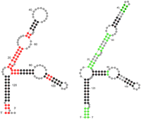
Two secondary structures for the 5S rRNA from the Archaeon, Methanothermobacter thermautotrophicus (strain δ-H; variant 2). (Left) The accepted phylogenetic structure (Szymanski et al. 2002). (Right) A minimum free energy (mfe) structure computed by UNAFold (Markham and Zuker 2008). Each base is drawn within a colored circle: (black circles) base pairs that are common to both structures, (red circles) base pairs in the phylogenetic structure that do not occur in the mfe structure, (green circles) base pairs in the mfe structure that are not in the phylogenetic structure, (gray circles) single-stranded bases.
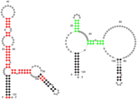
Two secondary structures for the 5S rRNA from the Archaeon, Haloarcula japonica. (Left) The accepted secondary structure computed by phylogenetic methods. (Right) A computed structure comprising base pairs that have probabilities >50%, computed by UNAFold (Markham and Zuker 2008). The coloring scheme is identical to that used in Figure 1, as is the total number of red (24) and green (11) circled base pairs. The BP distance between this pair of structures is 35, the same as the corresponding distance from Figure 1.
The necessity of a more discriminative method for comparing RNA secondary structures is what motivated the development of our comparative method—the relaxed base-pair (RBP) score. The RBP score generalizes the BP metric. It has a relaxation parameter, t ≥ 0, that indicates the degree of relaxation. We denote the RBP score between two secondary structures, S and S′, by ρt(S, S′). When t = 0, the RBP score is the same as the BP distance. When t = ∞ (i.e., very large), ρt(S, S′) = 0 if S = S′, and is 1 otherwise. Useful values of t depend on the length of the RNA and on the average number of base pairs in foldings.
RBP ILLUSTRATION
The RBP score can be explained in words with the aid of illustrations. Details appear later (Materials and Methods). A secondary structure can be represented as a “structure dot plot.” A base pair between the ith and jth ribonucleotides, ri and rj, respectively, where i < j, can be plotted as a “dot” or other symbol in row i and column j of a triangular matrix. Our convention is that the i (5′) index increases top to bottom, and the j (3′) index increases left to right. The distance between two base pairs is defined to be the maximum of the 5′ index difference and the 3′ index difference. For example, the distance between G23 • C94 and U30 • A86 is 8, because 30 − 23 = 7 and 94 − 86 = 8. Given two secondary structures, S1 and S2, the base pairs of S1 can be plotted with red dots and those of S2 with green dots. When a base pair is in both structures, a black dot is used. The BP metric counts the total number of red and green dots.
The RBP score, illustrated here with the relaxation parameter t = 1, is less strict. If the two structures are the same, all dots are black and the RBP score is set to 0. Otherwise, choose a red or green base pair that is the farthest away from a base pair of the opposite color (including, of course, black). Exclude it from further consideration. Then place a 1 × 1 square box centered about each base pair. With the exception of the excluded base pair, if every red or green box overlaps with or touches a box of the other color, including black, along an edge or at a single vertex, then the RBP score is set to 1. If this is not possible, then another red or green base pair is excluded, and then each square box is expanded to be 2 × 2. This process continues until d base pairs have been excluded, and each d × d square box of the nonexcluded base pairs overlaps with or touches a box of the opposite color. At this point, the RBP score is set to d.
We illustrate the computation of the RBP score by comparing the same pairs of structures that appeared in Figures 1 and 2 using a dot plot format. In Figure 3, the squares are 3 × 3 and the RBP score is 3. The three green base pairs closest to the diagonal and near (40,40) have been excluded, although one of them touches a black square. However, this base pair did not touch a red or black base pair when the squares were 2 × 2, so excluding two base pairs was insufficient. These three excluded base pairs are drawn using a darker shade of green in Figure 1. At a square size of 3 × 3, all the nonexcluded red or green base pairs are close to a base pair of the opposite color (or black).
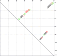
A structure dot plot that superimposes the phylogenetic structure of Methanothermobacter thermautotrophicus 2 5S rRNA (red and black squares) and a mfe structure for the same RNA (green and black squares). In this format, it is easy to visualize structural similarity. The squares are hollow to facilitate recognition of overlapping or touching squares. The squares are all 3 × 3.
Figure 4 superimposes the secondary structure pair from Figure 2 in dot plot format. In this case, the squares are 18 × 18. For this very large square size, there are 10 red squares that do not touch or overlap with a green or black square, and six green squares that do not touch or overlap with a red or black square. That is, there are 16 excluded base pairs. However, if the square size is reduced to 17 ×17, the number of excluded base pairs rises to a number >17, yielding an RBP score of 18.
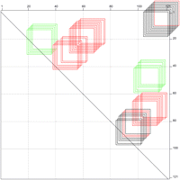
A structure dot plot that superimposes the phylogenetic structure of Haloarcula japonica (red and black squares) and a consensus structure for the same RNA (green and black squares).
If a base pair is in one structure and not in another, the BP metric does not take into account how close it might be to a base pair in the other structure. The BP metric uses a rigid measure of closeness. Two base pairs are “close” when they are the same. The RBP score uses a relaxed degree of closeness, so that two base pairs are “close” when the distance between them is within some threshold. Moreover, the threshold of closeness is flexible. Initially, the threshold is 0. However, as base pairs are excluded, the threshold grows in proportion to the number of excluded base pairs. The reason for doing this is to achieve a balance between the degree of closeness and the number of excluded base pairs, which can be regarded as outliers.
When the t parameter is not 1, the boxes in the dot plot are td × td in size after d base pairs have been excluded. When t = 0, the “boxes” become single base pairs so that base pairs are excluded until the remaining ones are in both structures. This shows that the RBP score is equivalent to the BP metric when t = 0. The RBP score can only remain the same or decrease as t increases. If t is set to the length of the sequence (a large number), then no base pairs are excluded if the structures are identical, so the RBP score is 0. Otherwise, after one base pair is excluded, the boxes are all t × t. They all intersect with one another, making the RBP score 1. That is, for t large enough, the RBP score reduces to a trivial case: 0 for identical structures, and 1 in all other cases.
COMPUTATIONAL RESULTS
Human mRNAs used for computations
Computations were performed on a selection of 13 human mRNA sequences of varying lengths (See Table 1). This collection overlaps the set used in a previous study (Ding et al. 2006). For each mRNA, 1000 foldings were computed by sampling from the Boltzmann distribution of all possible foldings. In addition, mfe structures were computed for each mRNA. All foldings were computed using the UNAFold package (Markham and Zuker 2008). Using different values of the t parameter, including t = 0 to reproduce the BP metric, RBP scores were computed for each of the (1000 × 999)÷2 pairs of structures for a given mRNA. Our results focus on the differences between the BP metric and RBP as seen for these mRNAs, using a variety of different computational tools.
Locus, gene name, and a brief description of the gene product for each of the 13 mRNA sequences used in our computations
Stability of clusters
Foldings were clustered using the spectral k-means clustering algorithm (Ng et al. 2001). The k-means clustering algorithm, the final step in the clustering process, is stochastic, meaning that cluster results differ when it is run several times on the same set of structures. Each clustering of 1000 structures was validated by taking random subsamples of size 100 and clustering them. The “Jaccard” score was used to measure the deviation of the subsample clustering to the way in which the same structures are grouped in the full 1000-structure clustering. This process was repeated a number of times to yield an average Jaccard score. Scores of 1 (maximum) indicate very stable clusterings and scores of 0 (minimum) indicate very unstable clusterings. Figure 5 shows line plots representing the clustering stability for each of the sequences. Red is used for the BP metric (t = 0) and blue for the RBP scores (t > 0). The RBP lines are almost always longer than the corresponding BP line, and are always longer for at least one value of t > 0. In addition, RBP scores often come close to the optimal value of 1. In some cases, the RBP scores appear “significantly” higher than the BP score. The subjective conclusion from these computations is that spectral k-means clustering works well with the RBP score and gives more stable clusterings when t > 0.
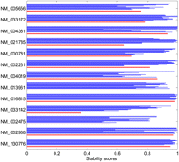
Clustering stability scores (horizontal axis) for the BP metric (t = 0, red) and RBP scores (t > 0, blue) for the 13 sequences listed (vertical axis, with sequences listed in order of length, shortest at the bottom). Stability scores approaching 1 indicate very stable clusters. The RBP relaxation parameters are t = 0.01, 0.02, 0.05, 0.1, 0.2, 0.5, 1, 2, 5, 10, and 20, corresponding to consecutive blue lines, bottom to top, respectively, for each sequence. Higher t values appear to give more stable clusters.
Computing representative foldings
The consensus secondary structure in Figure 2 contains, by definition, all base pairs whose probabilities in the Boltzmann distribution are >50%. It can be computed without using stochastic sampling. However, when structure samples are clustered, a consensus structure for each cluster is formed using the base pairs that occur in >50% of the foldings within the cluster. Such a structure is not contained in the sample, and it will vary somewhat each time the sampling process is repeated. When using the BP metric, the consensus structure is also a “centroid.” For any pairwise scoring method, such as RBP, a centroid of a cluster of foldings is a folding such that the sum of all the scores between it and all members of the cluster is minimized. When t = 0, the centroid is unique and equal to the consensus structure (Ding and Lawrence 2003). This pleasing attribute is lost when t > 0. The consensus structure, while still of interest, is no longer a centroid. Furthermore, we are unaware of any algorithm that would compute a true centroid. It is also clear that a centroid is no longer unique. As an example, when t is very large, any structure in a cluster is a centroid for the cluster and any other structure is not.
For this reason, we compute “medioids” for clusters. A medioid is a member of a cluster that minimizes the sum of scores between it and all (other) members of the cluster. It is not unique in general.
Medioids and mfe structures
The mfe structure is by definition the most probable structure, but for the mRNAs we considered, the probability of any particular structure in the Boltzmann ensemble is so small that one would never expect to find the mfe structure in a stochastic sample of 1000 structures. However, it is valid to ask if the mfe structure belongs to a highly probable cluster of similar structures. Previous work using the BP metric (Ding et al. 2005) showed that the mfe structure could belong to highly probable or less probable clusters. For each of the 13 mRNAs we studied, the mfe structure was computed and assigned to the nearest cluster. The nearest cluster to any given structure is the cluster whose medioid is closest to that structure, where structure closeness is the RBP score. The mfe structure Smfe is assigned to a cluster only if ρt(Smfe, Smedioid) does not exceed the maximal RBP score within the cluster, where Smedioid is the medioid structure. Otherwise, the mfe structure is considered to be an outlier sitting in a lone cluster. We define a dominant cluster to be one containing >70% of the structures, and a minor cluster to contain <10%. A large cluster is defined as nondominant, but containing at least 50% of the structures. Finally, a small cluster is nonminor and contains <50% of the structures.
The mfe structure is assigned to minor, dominant, and midsized clusters across the sequences. For some of the sequences, the assignment switches from one type of cluster to another as the t parameter changes. For NM_004381, the mfe structure is consistently assigned to a dominant cluster. The mfe structure is consistently assigned to a minor cluster for NM_002988. For NM_013961, the mfe is assigned to a minor cluster for six values of t and to a large cluster for the other six values of t.
Figure 6 shows bar plots for mRNAs NM_004381, NM_002988, and NM_013961. For NM_004381, the clustering is quite stable over the different values of t. For each value of t, a major and a small cluster are computed. For four values of t, an extra one or two very small minor clusters are computed. The major cluster varies somewhat in size and the mfe structure is consistently assigned to it. For NM_002988, the clustering itself changes dramatically for t = 0.1, 0.2, and 0.5. For the other values of t, a major and a minor cluster are computed, with some variation in size. The mfe structure is always assigned to the minor cluster. Examination of the underlying data reveals that the minor cluster that contains the mfe structure is stable over all values of t. It is the major cluster that is broken into multiple clusters when more than two clusters are computed. Both clustering and mfe structure assignment appear unstable for NM_013961. A detailed examination of which structures are assigned to various clusters reveals an interesting fact. The smallest minor cluster to which the mfe structure is assigned occurs when t = 0.02 and contains 48 structures. Without exception, each of these structures appear in an expanded minor cluster to which the mfe structure is assigned or else in a major cluster to which the mfe structure is assigned. In other words, there is a well-defined minor cluster that either expands into a larger minor cluster or is absorbed into a major cluster. The mfe structure is always assigned to the cluster containing these 48 structures. In other cases where mfe structure assignment appeared to be unstable, a careful analysis revealed a similar situation.
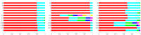
Bar plots for three of the 13 mRNAs: NM_004381 (left), NM_002988 (middle), and NM_013961 (right). Bar lengths indicate cluster sizes (horizontal axis), which sum to 1000. Different bars correspond to different values of the RBP relaxation parameter (t, vertical axis), which increase bottom to top. The colors are used only for visual effect. (*) The cluster, if any, to which the mfe structure is assigned.
Two-dimensional cluster plots
Each structure in a sample, {S1, S2, …, SN}, corresponds to a vector in an N-dimensional space, where N = 1000. The jth coordinate of the ith vector is ρt(Si, Sj). These vectors were subjected to spectral k-means clustering (see Materials and Methods). The resulting clusters are groups of secondary structures corresponding to clusters of points in a 1000-dimensional space. We used principal component analysis (PCA) (Jolliffe 2002) to project these vectors into two dimensions in a way that minimizes the differences between the distances in the original high-dimensional space and those in the two-dimensional plots. We refer to the resulting plots as PCA plots.
Figure 7 contains pairs of PCA plots for six different mRNAs. The plots on the left are for the BP metric (t = 0), while those on the right are for t = 1, except for the last two RBP plots (j and l) where t = 0.1. We refer to the plots on the left as BP plots, and those on the right as RBP plots. The details of these plots are described by looking at them in pairs.
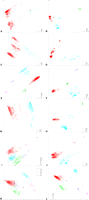
PCA plots for a variety of sequences and values of t. Colored crosses (×) indicate individual structures of the sample. The colors red, cyan, green, blue, magenta, orange, and gray correspond to the largest cluster, the next largest, and so on, respectively. Cluster sizes are shown in the boxed legends. (*) The mfe structure; (○ filled with the cluster color) cluster medioids. The number of clusters is computed automatically for each value of t. Each plot is labeled by LOCUS, t value: (A) NM_130776, 0; (B) NM_130776, 1; (C) NM_016815, 0; (D) NM_016815, 1; (E) NM_013961, 0; (F) NM_013961, 1; (G) NM_002231, 0; (H) NM_002231, 1; (I) NM_000781, 0; (J) NM_000781, 0.1; (K) NM_005656, 0; and (L) NM_005656, 0.1.
-
Plots A and B: The BP plot contains just two clusters, with the major one containing all but 38 of the sampled structures, while the RBP plot breaks up the sample into a dominant cluster, a small cluster, and a minor cluster. The dominant cluster in the BP plot looks like a union of two clusters (upper versus lower). We could have forced the creation of three clusters in this case, but this occurs automatically in the RBP plot. Moreover, the RBP plot shows a better separation of clusters.
-
Plots C and D: Both PCA plots have two clusters, and in both cases, the mfe structure is assigned to a dominant cluster. The RBP plot has compact clusters and avoids the intermingling of structures that appears in the BP plot. Note also that the mfe structure is very close to the medioid in the RBP plot, while this is not the case in the BP plot.
-
Plots E and F: The RBP plot contains a more compact dominant cluster than the BP plot. Two minor clusters from the BP plot (green and blue) are merged into a single cluster in the RBP plot (green). The smallest minor cluster in the BP plot (magenta) is retained in the RBP plot (blue). Both plots assign the mfe structure to equivalent minor clusters.
-
Plots G and H: The BP plot comprises two small clusters that are spread out and somewhat intermingled. The RBP plot contains a new minor cluster that is very well separated from the other two clusters. The large and small clusters (red and cyan, respectively) in the RBP plot are more compact than the two in the BP plot, and they are better separated. One can visualize drawing a straight line in the RBP plot that separates the two largest clusters. This cannot be done in the BP plot. The mfe structure, assigned to large clusters in both cases, appears closer to the cluster medioid in the RBP plot.
-
Plots I and J: The BP plot contains seven clusters, of which four are minor. The three large clusters and largest minor cluster seem well separated visually. The mfe structure is assigned to a minor cluster, but it nevertheless appears far from its own cluster medioid and very far from all the other cluster medioids. The RBP plot is for t = 0.1, which represents a very small degree of relaxation. There is a dramatic change. Only two clusters appear, well separated but with elongated “tails.” The “tail” of the major cluster appears to point to the mfe structure, which is assigned to it. This dramatic change illustrates how the BP metric can give results that are unstable. The RBP plots yield two or three clusters for t ≥ 0.1. Assignment of the mfe structure varies but a closer examination (data not shown) shows that cluster 5 of the BP plot is always completely absorbed into a cluster to which the mfe structure is assigned as t varies. As is the case with NM_013961 in Figure 6, there is a small cohort of structures that are always placed in the same cluster as t varies, and the mfe structure is always assigned to the cluster containing them, no matter what the size of the cluster.
-
Plots K and L: This is another case where changing t from 0 to 0.1 makes a dramatic difference. However, in this case, both plots contain five clusters. The point is that just a small degree of relaxation can result in greatly improved clustering. The RBP clusters, with the possible exception of the second largest, are more compact than those in the BP plot. Moreover, the RBP clusters are all well separated. The mfe structure assignment changes from minor to dominant, but in both plots, the mfe appears far from the cluster medioid. Although the number of RBP clusters increases to seven for t = 1 and then decreases to four for t = 10 (data not shown), mfe structure assignment is either to a dominant or a large cluster for t ≥ 0.05. We consider this to be a stable assignment. The large cluster to which it is assigned in the RBP plot shown is almost dominant.
Because we used a different clustering algorithm than Ding et al. (2006), our cluster sizes and mfe structure assignments for the BP metric (t = 0), in general, will differ from what they reported. Table 2 summarizes the cluster sizes and mfe structure assignments given in Figure 7 and compares them with equivalent computations reported by Ding et al. (2006). We consider our ρt results to be “correct” in the sense of being as good as possible using our methods. Differences that stand out the most are contradictory assignments of the mfe structure for the first and last two sequences in Table 2. However, our computations clearly confirm once more that the mfe structure need not belong to a highly probable group of structures and that it can be isolated in structure space.
A comparison of cluster sizes and mfe structure assignment
Medioid PCA plots
The use of the BP metric to cluster a sample of structures gives a single group of clusters and one medioid for each cluster. We saw that using the RBP score can result in the appearance of new clusters, and so we decided to compute medioids for all the different values of t used in this work and to display them all in a single PCA plot. Because these structures are medioids of clusters computed using many different values of t, we had to decide on some common scoring method to compare them. We chose the BP metric and were thus able to compute PCA plots. Figure 8 contains PCA plots of all the cluster medioids for four different mRNAs. In some cases, the medioids appear to aggregate into clusters of their own. For instance, the NM_130776 plot contains a cluster of medioids that includes a BP cluster medioid. In such a case, the BP metric was sufficient to identify a cluster, but the presence of RBP cluster medioids close to the BP medioid serves to reinforce the original BP cluster. On the other hand, isolated blue dots or small groups of blue dots far from any BP medioid (upper left of the NM_002231 plot) indicate clusters very different from what could be found using the BP distance alone.
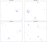
PCA plots of the cluster medioids derived by projecting medioid BP distances into two dimensions. The plots, clockwise from top left, are for NM_130776, NM_013961, NM_021785, and NM_002231. (Red circles) BP metric medioids, (blue dots) all the RBP medioids computed using various t ≠ 0 values.
Varying the relaxation parameter
At the beginning of this study, it was not at all clear what value or values of the relaxation parameter are appropriate for a particular RNA. Computations were performed for t = 0, 0.01, 0.02, 0.05, 0.1, 0.2, 0.5, 1, 2, 5, 10, 50, 100, and so on. The intent was to span the range of “useful values.” For the sequences we analyzed, values >50 produced little further variation and gave trivial 0 or 1 scores for the smaller sequences.
Individual plots of ρt versus t may sometimes suggest appropriate values of t. Figure 9 shows the decrease of ρt with increasing t for the two pairs of 5S rRNAs depicted in Figures 1 and 2. Both scores are identical for the BP metric, t = 0, but the score for the M. thermautotrophicus pair initially decreases sharply with t, while the score for the Haloarcula japonica pair does not. For the first pair, values of t < 0.2, where the score is 10 and values of t > 1, where the score is 3, appear intuitively to be inappropriate. The score falls dramatically up to t = 0.2, while beyond 1 there is scarcely any further improvement. If we choose a subjective rule of not increasing t beyond the “point of diminishing returns,” then t = 1 is an appropriate choice. For the second pair, there is a gradual decrease in the score as t increases. Visually, there appear to be no “appropriate values” for t that stand out. The subjective rule cannot be applied for all sequences.
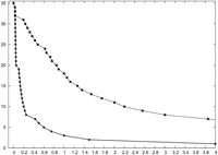
RBP scores (vertical axis) are plotted versus different relaxation parameters (horizontal axis) for two pairs of 5S rRNA secondary structures. (Solid line with circles) ρt(Sphylo, Smfe) versus t, where Sphylo and Smfe are the phylogenetic and mfe structures for M. thermautotrophicus, respectively. (Dashed line with boxes) ρt(Sphylo, Sconsen) versus t, where Sphylo and Sconsen are the phylogenetic and consensus structures for H. japonica, respectively. Values of t are automatically chosen for each plot so that every possible RBP score occurs within the range 0 ≤ t ≤ 4. The RBP score reaches its minimum value of 1 for the M. thermautotrophicus pair when t = 4, so that 35 circles appear in the plot. The two plots coincide for the first four (identical) values of t.
In our quest to find appropriate values of t that could be used for all pairs of structures in a sample, we decided to investigate how RBP scores deviate from the BP metric as t increases. For this purpose, we employed the nonparametric Kendall τ statistic (see Materials and Methods). For a particular structure, Si, the RBP scores create a ranking of all the structures in terms of increasing values of ρt(Si, Sj) for different js. The value of τ lies between 1 and −1, where 1 would occur if the rankings are identical and −1 indicates a total reversal. If two rankings are random and independent of one another, then the expected value of τ is 0. The Kendall τ statistic measuring the change in rankings between ρ0 and ρt is denoted by τt(i). Finally, τt was defined as the average value of τt(i) over all the structures. This statistic measures the overall change in rankings as t varies.
Figure 10 plots the average τt scores for the deviation from the BP metric as t increases from 0. They all decrease from 1 to 0 (or a slightly negative value). The decrease appears to be “somewhat linear” for middle values of t. We found no relation between sequence length and the rate of decrease.
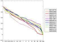
Average Kendall τ ranking scores (vertical axis) for the BP metric versus ρt plotted for different values of t (horizontal axis). The legend lists the sequences in order of length (shortest at the bottom). Dashed lines are used for the average τt scores for NM_033172 (pale green) and NM_033142 (red) because they exhibit, to some extent, the most extreme behavior. The scores were evaluated only for the values of t indicated along the horizontal axis, and straight lines were used to connect successive values of τt. No inference can be made on the behavior of τt between adjacent values of t.
For the ranking of 1000 items, a Kendall τ value of 0.07 or larger will occur by chance just 0.1% of the time if the rankings are totally uncorrelated (Sheskin 2007). What Figure 10 shows unambiguously is that for values of t that we would consider using in constructing clusters, say between 0.02 and 20, ρt is significantly different from the BP metric, but not so different as to be totally dissociated from it.
DISCUSSION
We began this work with two goals in mind. One was to group large numbers of foldings of an RNA sequence into a small number of well-separated clusters. The second was to compute an appropriate secondary structure to represent each cluster. The RBP score was designed to be an improvement on the BP metric (Ding et al. 2005). We coupled this new scoring method with powerful clustering algorithms that have not, as far as we know, been used previously in clustering RNA secondary structures.
We were deliberate in not using hierarchical clustering (Johnson 1967; Manning et al. 2008) or the related neighbor-joining algorithm (Saitou and Nei 1987) to compute clusters of structures, even though such methods are simple to use and readily available (Felsenstein 1989). An underlying assumption of these algorithms is that the data are related by a tree that the algorithm (re)constructs as best it can. Such computations are inappropriate for our purposes. We are not comparing homologous or orthologous RNA structures on different RNA sequences, for which tree construction is appropriate.
Other comparison methods
Numerous articles have been published over the years describing different approaches for comparing RNA secondary structures (Shapiro 1988; Shapiro and Zhang 1990; Moulton et al. 2000; Giegerich et al. 2004; Ding et al. 2005; Steffen et al. 2006; Liu et al. 2008). Viewing RNA secondary structures as trees and the use of tree edit algorithms to measure the difference between structure pairs was introduced ∼20 yr ago (Shapiro and Zhang 1990). Tree edit algorithms tend to be slow, and in the past, computational complexity led to the use of heuristics that did not guarantee optimal solutions. In the context of RNA secondary structures, M base pairs would correspond to (at most) M nodes in a tree, and it is now known that such algorithms can run with a time and space complexity of O(M3) (Demaine et al. 2007). While practical for comparing a limited number of structures, this sort of cost is prohibitive if the goal is to compute distances for all N(N−1)÷2 pairs of structures in a sample of N structures. Other methods, including tree edit algorithms, are more suitable for comparing structures on different RNAs. In our opinion, the RNAshapes algorithm (Giegerich et al. 2004; Steffen et al. 2006) stands out as a useful tool for reducing huge numbers of possible structures to a smaller number of “shapes” together with actual secondary structures. At this time, it is not clear to us how to compare RNAshapes with our methods.
Computational and technical considerations
Unlike the BP metric, the RBP score is not in general a metric for t > 0. Although obviously symmetric, it sometimes fails the triangle inequality. For the purpose of deriving clusters and projecting into lower dimensions for display purposes, our computations were based on embedding RBP scores into high-dimensional Euclidean spaces, where the triangle inequality is satisfied.
The RNA structures in a sample will have different numbers of base pairs. Suppose that structure S1 has M1 base pairs and that structure S2 has M2 base pairs. The BP score between these two structures can be computed in O(M1 + M2) time by a simple scan of all the M1 base pairs in the first structure, counting base pairs that do not occur in the second structure. A second scan is performed on the M2 base pairs in the second structure. That is, computation time is linear in the total number of base pairs. This is no longer the case when computing ρt for t > 0. It appears at first that all M1 base pairs in one structure must be compared with all M2 base pairs of the other to compute the list of distances required to compute ρt. This yields a time complexity of O(M1M2). However, the base pairs of structure S1 may be “sorted” in two dimensions by the construction of a 2-d tree using the K-d tree method (Bentley 1990). Computation time is O(M1 log M1). For each base pair in S2, the closest base pair in S1 may be found in O(log M1) steps. Computing all the closest base pairs then requires O[(M1 + M2)log M1] steps, including the tree construction. Similarly a 2-d tree is computed for S2, and nearest base pairs in S2 are computed for base pairs in S1. The entire process requires O[(M1 + M2)(log M1 + log M2)] steps. This is equivalent to O[(M1 + M2)log (M1 + M2)] steps.
As stated above, there are N(N−1)÷2 distinct pairs of structures in a sample of N structures, so that ρt must be computed for a huge number of structure pairs. In practice, this computation can become the bottleneck if done naively. Fortunately, the total number of distinct base pairs in a sample tends to be much lower than the number of structure pairs. The total number of distinct base pairs is observed to be a “small” multiple of the sequence length, where “small” ranges from 1.8 to 4.9 (3.7 ± 0.9) for the mRNAs analyzed in this work (Table 1). Thus, the entire computation could be performed by creating a 2-d tree for each structure, and searching each tree for the nearest base pair to each distinct base pair.
Choosing the relaxation parameter
In our opinion, the Kendall τ plots in Figure 10 serve to reassure us that values of t centered at 1 and varying between 1/c and c for c = 20 give useful results. One possibility for choosing t objectively would be to compute an average Kendall τ plot routinely before computing clusters. This plot would then be used to select a value of t that corresponds to a target value of τ, say somewhere between 0.5 and 0.7, thereby ensuring that the RBP scores do not deviate entirely from the BP metric, but that there is enough relaxation induced by the selected t to render RBP rankings sufficiently different from BP rankings. Although choosing a target value for τ is itself subjective, choosing t in this manner would be automatic and would not rely on human intervention.
Another solution to the problem of choosing t would be to eliminate choice by integrating the RBP score over all t. A second glance at Figure 9 suggests computing the “area under the curve” from t = 0 to the value of t where the RBP score becomes 1. For the M. thermautotrophicus pair of structures, ρ1 = 3, while the area under the curve is 11.3. For the H. japonica pair, ρ1 = 18, and the area under the curve is 107.9. The ratio of the ρ1 scores is 3/18 ≈ 0.17 and the ratio of the two areas is 11.3/107.9 ≈ 0.10. They agree within a factor of 2.
Conclusions and future work
Our preliminary study of the novel RBP algorithm coupled with spectral k-means clustering has provided us with results that are compelling enough to instigate further investigation. With a properly chosen relaxation parameter, t, the RBP score yields a more biologically meaningful measure of the difference between two secondary structures on the same RNA. Computing clusters as described yields better defined, more compact, and better separated clusters than previously reported methods. In addition, when the mfe structure is assigned to a cluster, it is often placed close to the medioid structure when viewed in a PCA plot.
We intend to implement efficient computation of RBP scores as described above in order to incorporate clustering and medioid prediction into the UNAFold software package (Markham and Zuker 2008), into the existing mfold web server (Zuker 2003), and into future updated web servers. Consensus structures, although not centroids, are still important and will be computed for individual clusters by using base pairs that occur in over half the structures in a cluster.
We will pursue the question of computing appropriate values of t using the Kendall τ statistic and will also experiment with averaging over t. Our intuition is that computing with a single appropriate value of t will give sharper results than averaging over t. In any case, more computations need to be performed on different classes of RNA, including structural and noncoding RNA. Another approach will be to compute medioids for many values of t and cluster them. The relatively small number of medioids in Figure 8 were not clustered. This computational experiment may help to determine which clusters are genuine (stable over a range of relaxation parameters) and which are more akin to noise.
MATERIALS AND METHODS
Algorithms and statistical methods
The RBP algorithm
Denote a base pair between ribonucleotides i and j by i·j. The distance between two base pairs i·j and i′·j′ is defined by (Zuker 1989b) The distance, δbs, between a base pair, i·j, and a structure, S, is defined as the smallest distance between i·j and a base pair in S. That is,
 For two structures, S1 and S2, containing M1 and M2 base pairs, respectively, a total of M1 + M2 distances are computed: all M1 distances between the base pairs of S1 and the structure S2 and all M2 distances between the base pairs of S2 and the structure S1. These distances are by no means distinct. In particular, if S1 and S2 have M3 base pairs in common, then 0 will occur M3 times. These distances are sorted, with repeats, in decreasing order. We denote these sorted distances by {Δ1, Δ2, …, ΔM1 + M2}, where Δi ≥ Δj if i < j. For a relaxation parameter t ≥ 0, we define
 This method of setting a flexible threshold of significance was inspired by the Prokhorov algorithm (Prokhorov 1956). Note that if t = 0, then tm is always 0, so that ρ0(S1, S2) is the number of nonzero distances, which is the BP score. If t > max Δi, then the condition is satisfied for m = 1, so the RBP score is 1 if the structures are different and 0 if they are identical. The sensitivity of the RBP algorithm
can be manipulated using the t parameter. Changing t alters the threshold for significant differences. It is clear that for a fixed pair of structures, ρt(S1, S2) is nonincreasing as t increases. Note that the computational cost for calculating the RBP scores for multiple values of t is minimal once the list of M1 + M2 distances is computed and sorted. RBP scores can easily be calculated for various t values by simply scanning the distances from largest to smallest.
This method of setting a flexible threshold of significance was inspired by the Prokhorov algorithm (Prokhorov 1956). Note that if t = 0, then tm is always 0, so that ρ0(S1, S2) is the number of nonzero distances, which is the BP score. If t > max Δi, then the condition is satisfied for m = 1, so the RBP score is 1 if the structures are different and 0 if they are identical. The sensitivity of the RBP algorithm
can be manipulated using the t parameter. Changing t alters the threshold for significant differences. It is clear that for a fixed pair of structures, ρt(S1, S2) is nonincreasing as t increases. Note that the computational cost for calculating the RBP scores for multiple values of t is minimal once the list of M1 + M2 distances is computed and sorted. RBP scores can easily be calculated for various t values by simply scanning the distances from largest to smallest.
Spectral k-means clustering
Clustering of secondary structures was performed using the spectral k-means clustering algorithm (Ng et al. 2001). This algorithm employs the k-means clustering algorithm (Lloyd 1982), which is stochastic. The exact algorithm is as follows:
-
Let {S1, S2,…, SN} be a sample of N secondary structures on the same RNA molecule. Fix some relaxation parameter, t. For structure i, define a vector
 in N-dimensional Euclidean space by
-
For a suitable σ > 0, which is chosen automatically by the algorithm, define an N × N affinity matrix, A = (aij), by

-
Construct a scaled matrix, L = D−1/2 AD−1/2, where D is a diagonal matrix defined by

-
If the N eigenvalues of L are ordered as λ1 ≥ λ2 …, then for any K between 1 and N, form an N × K matrix, X, where the K columns of X are orthonormal eigenvectors of L corresponding to the λ1, λ2,…,λK, respectively.
-
Define the projected feature space, Y, to be the N × K matrix formed from X by normalizing the rows of X to unit length. Each secondary structure is now represented by a row in Y, which is a point in K-dimensional Euclidean space, ℝK.
-
Use k-means clustering on these N points in ℝK to cluster them into K clusters.
In the above, only step (1) is specific to our application. Note that in the definition of aij,  is used. This is
 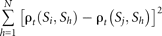 , not ρt (Si, Sj)2. In general, the number of points to be clustered and the lengths of the vectors are not the same.
The Calinski and Harabasz (CH) index
The algorithm described above creates a specified number of clusters. It does not choose K, the number of clusters. A good clustering is one that forms closely knit clusters that are far apart from each other. The
Calinski and Harabasz (CH) index (Calinski and Harabasz 1974) provides some measure of this. Ding et al. (2005) successfully used the CH index to choose K. Given N objects clustered into K groups, the CH index is defined to be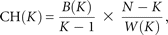 where B(K) are the between-cluster sums of squares and W(K) are the within-cluster sums of squares. The CH index does not have a global maximum and therefore a search space must be
defined for K ≥ 2 (the index is undefined for K = 1). We use the CH index to determine an optimal number of clusters within the range of 2–15.
where B(K) are the between-cluster sums of squares and W(K) are the within-cluster sums of squares. The CH index does not have a global maximum and therefore a search space must be
defined for K ≥ 2 (the index is undefined for K = 1). We use the CH index to determine an optimal number of clusters within the range of 2–15.
The Jaccard similarity coefficient
The Jaccard index (Jaccard 1901) was used to measure the consistency of clusterings obtained by the k-means algorithm. Given a clustering C(K) of 1000 structures into K groups, we measure the clustering stability by randomly subsampling h structures from the 1000 structures and clustering them separately into K groups to form the clustering Ch′(K). This clustering is then compared to their clustering Ch(K) in C(K) using the Jaccard index as a measure of similarity. The Jaccard index is typically used to compare two clusterings and is
defined to be the ratio [N11/(N11 + N10 + N01)], where N11 is the number of point pairs grouped together in both clusterings, and N10 and N01 are the number of point pairs grouped together in one clustering but not the other. Identical clusterings have a Jaccard
index of 1. Therefore, using this as a measure of similarity J[Ch′(K), Ch(K) between the two clusterings for the subsampled h points, and repeating our subsampling n times, the stability score is defined to be The resulting stability score is a number between 0 and 1, with stable clusterings having a score that approaches 1.
Kendall's τ statistic
Kendall's τ (Kendall 1975) is a nonparametric statistic that is used to compare two different rankings of the same objects. Given two rankings (orderings)
of N objects, ra and rb, a pair of items in the rankings is defined to be concordant if both rankings agree on how the items are ordered. Otherwise,
the pair is said to be discordant. The items represented in the rankings are compared pairwise and a count of the concordant
pairs P and discordant pairs Q is taken. Kendall's τ is defined to be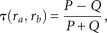 where τ → 1 as the rankings become identical, and τ = −1 corresponds to a complete reversal of rankings. In the context of
this work, there are N (1000) secondary structures, (S1, S2,…, SN), in a sample. Any particular structure, Si induces a ranking, ri,t, on the N − 1 remaining structures determined by increasing values of ρt(Si, Sj). Let τt(Si) be defined for the rankings ri,0 and ri,t. Finally, compute the average of all the τt(Si),
where τ → 1 as the rankings become identical, and τ = −1 corresponds to a complete reversal of rankings. In the context of
this work, there are N (1000) secondary structures, (S1, S2,…, SN), in a sample. Any particular structure, Si induces a ranking, ri,t, on the N − 1 remaining structures determined by increasing values of ρt(Si, Sj). Let τt(Si) be defined for the rankings ri,0 and ri,t. Finally, compute the average of all the τt(Si), We call τt the rank score and use it to compare the BP metric to RBP scores as t varies. If two rankings of N objects are stochastically independent, then the associated statistic,
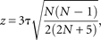 converges to the normal distribution with mean 0 and variance 1 [N (0,1)] as N → ∞ (Sheskin 2007). In practice, z is almost identical to N(0,1) when N > 40. For N > 40, significance levels for Kendall's τ statistic can be computed using readily available tables for the normal distribution.
ACKNOWLEDGMENT
We thank the reviewers for their critical remarks and helpful suggestions.
Footnotes
-
Reprint requests to: Michael Zuker, Department of Mathematical Sciences, Rensselaer Polytechnic Institute, Troy, NY 12180, USA; e-mail: zukerm{at}rpi.edu; fax: (518) 276-4824.
-
Abbreviations: mfe, minimum free energy; BP, base pair (in the context of base-pair metric or base-pair score); RBP, relaxed base pair (score).
-
Article published online ahead of print. Article and publication date are at http://www.rnajournal.org/cgi/doi/10.1261/rna.903510.
-
- Received December 24, 2009.
- Accepted February 3, 2010.
- Copyright © 2010 RNA Society