betAS: intuitive analysis and visualization of differential alternative splicing using beta distributions
- Mariana Ascensão-Ferreira1,3,
- Rita Martins-Silva1,3,
- Nuno Saraiva-Agostinho2 and
- Nuno L. Barbosa-Morais1
- 1Instituto de Medicina Molecular João Lobo Antunes, Faculdade de Medicina, Universidade de Lisboa, Lisboa 1649-028, Portugal
- 2European Molecular Biology Laboratory, European Bioinformatics Institute, Wellcome Genome Campus, Hinxton, Cambridge CB10 1SD, United Kingdom
- Corresponding author: nmorais{at}medicina.ulisboa.pt
-
↵3 These authors contributed equally to this work.
-
Handling editor: Javier Caceres
Abstract
Next-generation RNA sequencing allows alternative splicing (AS) quantification with unprecedented resolution, with the relative inclusion of an alternative sequence in transcripts being commonly quantified by the proportion of reads supporting it as percent spliced-in (PSI). However, PSI values do not incorporate information about precision, proportional to the respective AS events’ read coverage. Beta distributions are suitable to quantify inclusion levels of alternative sequences, using reads supporting their inclusion and exclusion as surrogates for the two distribution shape parameters. Each such beta distribution has the PSI as its mean value and is narrower when the read coverage is higher, facilitating the interpretability of its precision when plotted. We herein introduce a computational pipeline, based on beta distributions accurately modeling PSI values and their precision, to quantitatively and visually compare AS between groups of samples. Our methodology includes a differential splicing significance metric that compromises the magnitude of intergroup differences, the estimation uncertainty in individual samples, and the intragroup variability, being therefore suitable for multiple-group comparisons. To make our approach accessible and clear to both noncomputational and computational biologists, we developed betAS, an interactive web app and user-friendly R package for visual and intuitive differential splicing analysis from read count data.
Keywords
- beta distributions
- visual decision support tool
- differential alternative splicing
- multiple-group comparisons
INTRODUCTION
Species with similar numbers of protein-coding genes can have markedly discrepant numbers of functional proteins (Lee and Rio 2015). Alternative splicing (AS) greatly amplifies transcriptomic diversity through the production of several RNA isoforms from a single gene. Virtually all human protein-coding genes undergo AS (Pan et al. 2008) that expands the potentially functional transcriptome (Lee and Rio 2015) and contributes to the pretranslation regulation of gene expression (Irimia and Blencowe 2012).
Developmental stage- and tissue-specific transcriptomes are fine-tuned through the highly regulated usage of AS variants (Gallego-Paez et al. 2017), and perturbations in the physiological regulation of tissue-specific AS have been reported in disorders with different etiologies, such as autism (Irimia et al. 2014), myotonic dystrophy (Llorian and Smith 2011), and cancer (Dvinge and Bradley 2015). Moreover, splicing modulation has been therapeutically used to direct AS toward protective isoforms. Therefore, soundly quantifying AS and differences in splicing between conditions not only helps to elucidate molecular bases of tissue physiology, but can also reveal therapeutic targets (Effenberger et al. 2016; Havens and Hastings 2016).
High-throughput sequencing of RNA (RNA-seq) allows unprecedented precision in AS quantification (Pan et al. 2008). Computational tools developed for the identification and quantification of differentially spliced genes from RNA-seq data can be classified into isoform-resolution or count-based approaches (Pachter 2011; Liu et al. 2014). While isoform-resolution methods, also called “multiread” models (Pachter 2011), aim at directly estimating the relative abundances of full-length transcripts in each sample (Liu et al. 2014; Mehmood et al. 2019), count-based methods aim at detecting differential usage of local features (e.g., exons) rather than the whole gene, based on the number of RNA-seq reads unambiguously assigned to each unit (Pachter 2011; Liu et al. 2014; Mehmood et al. 2019). Counting units refer to splicing events, that is, gene regions showing local variation at the mRNA level due to two possible splicing outcomes, such as the inclusion or skipping of an alternative exon (Alamancos et al. 2014). A widely used metric for quantifying the fraction of mRNA isoforms that include an alternative sequence is the percent or proportion spliced-in (PSI), given by the ratio between inclusion and the sum of inclusion and skipping reads (Wang et al. 2008). For instance, AS quantification programmes rMATS (Shen et al. 2014), vast-tools (Tapial et al. 2017), Whippet (Sterne-Weiler et al. 2018), SUPPA2 (Trincado et al. 2018), MAJIQ (Vaquero-Garcia et al. 2016), and MISO (Katz et al. 2010) use PSI or analogous metrics for quantifying inclusion of alternative sequences.
Most differential AS analysis tools build on knowledge from differential gene expression analysis and apply linear modeling to define differentially spliced events between two or more groups (limma [Ritchie et al. 2015], edgeR [Robinson et al. 2010], DEXSeq [Anders et al. 2012], JunctionSeq [Hartley and Mullikin 2016], PennDiff [Hu et al. 2018], and DJExpress [Gallego-Paez and Mauer 2022]), while others quantify the difference of inclusion levels based on geometric distances between gene-level vectors (SplicingCompass [Aschoff et al. 2013] and DIEGO [Doose et al. 2018]). However, most of these approaches have limited applicability to the typical small sample sizes used in biomedical research. MISO's differential splicing approach relies on a probabilistic model that applies Bayesian statistics to isoform expression levels and thereby provides confidence intervals for PSI estimates for individual samples. However, MISO does not support multiple biological replicates directly.
Differential splicing analyses with small sample sizes should be supported by a compromise between modeling the uncertainty in the estimation of inclusion levels of AS events in individual samples and accounting for the biological variability among replicates. Although most tools overlook this compromise, rMATS’ (Shen et al. 2014) reportedly robust quantification pipeline (Liu et al. 2014) implements it by modeling: (i) the uncertainty in the estimate of alternative sequence inclusion in individual replicates as a function of the total number of supporting RNA-seq reads, assuming these follow a binomial distribution; and (ii) the variability of such inclusion level across biological replicates as random effects in a mixed model. Similarly, vast-tools (Tapial et al. 2017), Whippet (Sterne-Weiler et al. 2018), and MAJIQ (Vaquero-Garcia et al. 2016) use the beta distribution to model the PSI variance in a read coverage-dependent way. SUPPA2 (Trincado et al. 2018) also incorporates biological variability into the quantification of differential AS by ranking inclusion differences based on how extreme they are with respect to the average transcript abundance they are associated with.
Yet, such tools, although of straightforward use to bioinformaticians, are not easily usable by and fully intelligible to noncomputational scientists and/or lack interactive graphical frameworks allowing them to understand the statistics accommodating the two aforementioned sources of uncertainty, such that they can, for instance, critically evaluate discrepancies in consistency and reproducibility across differential AS analysis tools (Mehmood et al. 2019).
Therefore, we developed betAS, a user-friendly R package available via a web app that, from splice junction read counts obtained from vast-tools (Tapial et al. 2017), rMATS (Shen et al. 2014), or Whippet (Sterne-Weiler et al. 2018), allows intuitive analysis and visualization of differential AS based on beta distributions. As mentioned, beta distributions are suitable to provide the estimated probability distributions of PSIs from the evidence for inclusion or skipping of alternative sequences given by read counts, such that each beta distribution has the observed PSI as its mean and is narrower when read coverage is higher. While the precision of AS estimates (PSIs) modeled with beta distributions is therefore proportional to the associated coverage and reflected on the significance of AS differences between samples, plotting the estimated beta distributions provides an intuitive graphical framework for evaluating the compromise between the uncertainty in individual sample estimates and the variability among replicates. Likewise, betAS thrives as a decision support system that helps the user to judge which AS changes are biologically relevant and robust, rather than using context-independent predefined cutoffs.
The betAS visual interface is designed to be used by any scientist, irrespectively of their prior knowledge of R, and simplifies the analysis of user-provided tables with AS quantifications, as well as the ranking of differentially spliced events by a significance metric that incorporates information on the precision of the relative transcript abundances and that is suitable for multiple-group comparisons. This feature, to our knowledge absent in the best-established differential AS tools, is useful, for example, when studying the tissue- or differentiation stage-specific regulation of AS, as illustrated below in Results.
The betAS web app is available at https://compbio.imm.medicina.ulisboa.pt/betAS.
RESULTS
Beta distributions model PSI levels and associated confidence
Profiling AS from an RNA-seq-derived transcriptome relies on sampling the mRNA molecules present in the studied tissue at a given moment. RNA-seq reads that map to annotated exon–exon or exon–intron junctions are typically used as supporting evidence for either the inclusion or exclusion of alternative sequences in transcripts. The relative inclusion level of a known alternative sequence in a biological sample can be conveniently modeled by the beta distribution, with shape parameters given by the number of inclusion and exclusion reads (Fig. 1; Supplemental Fig. S1; see Materials and Methods; Katz et al. 2010; Shen et al. 2014; Vaquero-Garcia et al. 2016; Han et al. 2017; Sterne-Weiler et al. 2018), with the precision of the inclusion level estimate being therefore proportional to the number of supporting reads.
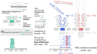
Beta distributions model PSI levels and associated confidence. Explanatory diagram of the estimation of the PSI with the beta distribution for an alternative transcript sequence (exon) of interest (green) from the RNA-seq junction read counts supporting the sequence's inclusion (inc) or exclusion (exc). The ability of the beta distribution to incorporate the mean value and the confidence of the PSI is further illustrated for two discrepant scenarios of read coverage: lower, with 10 reads (blue), and higher, with 1000 reads (salmon). PSIs randomly generated from the respective beta distributions (500 colored vertically “jittered” points per distribution and associated solid density lines) are dispersed around mean values, being less dispersed as coverage (i.e., confidence associated with supporting evidence) increases. Colored 95% confidence intervals for a proportion's test with P (in this case, PSI) equal to 0.8, with 10 (blue) or 1000 (salmon) trials. Colored (green/blue/salmon) squircles: alternative exons; gray squircles: constitutive exons; junction read depictions colored according to their exon coverage.
As shown in Figure 1, for a particular AS event the PSI quantification alone provides no information on the total number of supporting RNA-seq reads but only on the proportion of them providing evidence for inclusion. The two depicted AS events have contrasting numbers of reads supporting inclusion/exclusion (8/2 for the lower coverage example in blue, 800/200 for the higher-coverage case in salmon) but show the same PSI value. However, the stronger evidence provided by higher coverage (salmon) confers more confidence to its PSI estimate than to that of a case with lower coverage (blue), as illustrated by their confidence intervals (Fig. 1).
betAS pipeline enables intuitive visualization of the magnitude and significance of alternative splicing changes
To provide a decision-support tool for the analysis of AS differences between conditions, allowing subsequent interpretation of their biological implications, betAS implements intuitive visuals that incorporate the estimated inclusion levels and their precision.
AS is more prevalent and more conserved, across vertebrates, in nervous system tissues (Barbosa-Morais et al. 2012; Merkin et al. 2012). Moreover, neuronal-specific RNA-binding proteins that regulate AS in neurons contribute to the functional complexity of neurodevelopmental processes (Licatalosi and Darnell 2006; Raj and Blencowe 2015). Given this relevance of AS in neuronal specification, as a case study, betAS was applied to the analysis of AS changes during the transition from pluripotency to mature neuronal function in mouse by comparing the transcriptomes of samples in the extremes of the publicly available murine neuronal differentiation time line (Hubbard et al. 2013): embryonic stem cells (ESCs) and mature neurons (28 d in vitro).
Volcano plots illustrating the effect size/significance relationship for PSI differences across AS events are shown in Figure 2C,D. In this example, the selection of events differentially spliced between the two conditions aims to maximize both the probability of their PSI values being greater in one of the conditions and the actual difference in PSI between the two conditions. Thus, higher values of Pdiff and lower values of FPR highlight more robust separations between the estimated distributions of PSI (Supplemental Figs. S2 and S3), while greater effect sizes (ΔPSI) suggest stronger impacts on sequence inclusion of the biological differences between conditions.
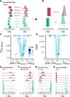
betAS pipeline enables intuitive visualization of AS changes. (A,B) Beta distributions (vertical “jitter” and density plots of the emitted values) illustrating PSI dispersion for each sample (A) and per phenotypic group (B), with the vertical dashed lines indicating the median PSI for each group, PSIneurons (dark red) and PSIESC (green). (C,D) Volcano plots illustrating the effect size (ΔPSI) as the difference between the median group PSIs and their significance assessed by the estimated probability of differential AS, based on the proportion of differences between ESC and neurons beta distribution randomly emitted values that are >0 (Pdiff) (C), and by the false positive rate (FPR) (D). Events are colored by the F-statistic, that is, the ratio of between- to within-group PSI variations (see Materials and Methods). Both y-axis scales are log-transformed to facilitate visualization. Upper row of trimmed points represents Pdiff > 0.9995 and FPR < 0.0001. (E–H) Beta distributions (density plots of the emitted values) and vast-tools’ PSIs (bottom, colored ticks) for selected events illustrative of different combinations of effect size and significance of AS differences, identified by vast-tools’ IDs (VAST-DB annotation for the mouse mm10 genome assembly): (E) MmuEX0003638 (gene Actn4, chr7:28895121–28895180), (F) MmuEX0001385 (gene 4833439L19Rik, chr13:54564515–54564621), (G) MmuEX0012381 (gene Commd6, chr14:101640288–101640299), and (H) MmuINT0085965 (gene Kctd17, chr15:78436995–78438486). (ESCs) Embryonic stem cells.
betAS allows the interpretation of ΔPSI values associated with different PSI/coverage scenarios. For instance, while the selected Gon4l exon (Fig. 2A,B) is barely more included in neurons than in ESCs, the volcano plot illustrates some stronger and more robust AS changes (Fig. 2C,D), with several AS events showing switch-like behaviors, as seen by extreme differences (i.e., close to absolute values of 1) in PSI between neurons and ESCs (Fig. 2C,D). Some of these AS changes are illustrated in Figure 2E–H, where the visualization of the beta distributions that model sample-wise inclusion levels elucidates on the differences at the PSI levels and their precision across samples. Among them, the two most extreme examples in significance and effect size, with absolute ΔPSI values >0.50, are exon MmuEX0003638 in gene Actn4, rarely included (PSI ≈ 0) in ESC but typically included (PSI ≈ 0.70) in mature neurons (Fig. 2E) and in neuronal tissues (https://vastdb.crg.eu/event/MmuEX0003638@mm10), and intron MmuINT0085965 in Kctd17, that shows high retention levels in ESC (PSI ≈ 0.75) and is spliced out (PSI ≈ 0) in neurons (Fig. 2H). In both cases, there are coverage differences (associated with differences in gene expression) between the two conditions, reflected by the different widths of the respective beta distributions (Fig. 2E,H). Visualization of inclusion levels through density plots of the respective beta distributions together with the usage of associated significance metrics such as the Pdiff also allows the user to spot outlier replicates, as for exon MmuEX0012381 in Commd6 (Fig. 2G), nearly constitutively included (PSI ≈ 1) in all ESC samples except one (PSI ≈ 0.2). Although showing an average ΔPSI similar to that of the intron retention event in Figure 2H, its Pdiff significance is penalized due to that inconsistency between replicates (Fig. 2C).
Assessment of betAS ability to estimate differential AS on simulated RNA-seq splice junction read counts from empirically derived PSI and coverage values
In order to benchmark betAS’ accuracy in quantifying differential AS, it should be tested on simulated RNA-seq junction read counts, such that the ability of the ΔPSI values estimated with betAS from the simulated reads could be compared with “ground truth,” reference ΔPSI values. Therefore, the biological and technical variability in PSI and read count distributions and their association with the sequencing sampling, together with the features of beta and Poisson distributions, were explored to simulate RNA-seq spliced junction read counts inspired in a real biological data set (see Supplemental Methods).
Large-scale AS quantifications available from GTEx (Lonsdale et al. 2013) were used to simulate “biology-inspired” PSI values (Fig. 3A; see Materials and Methods). To simulate PSIs reflecting the natural inclusion patterns of highly regulated AS events, the focus was on (i) tissues with prevalent and functionally relevant AS (muscle and brain); and (ii) AS events with typical inclusion levels that are lowly variable in samples of the same tissue, properties that find a proxy in the mathematical concept of unimodality of a distribution. For each representative tissue-unimodal AS event, junction read counts were simulated for a set of N replicates from PSI/coverage pairs.
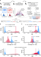
betAS accuracy in measuring PSI differences from simulated read counts. (A) Explanatory diagram of the implemented approach to simulate empirically inspired RNA-seq junction read counts. Reference PSI (PSIREF) and coverage (covREF) values for 563 muscle (red) and 309 cerebellum (blue) samples in GTEx version 7 are used to generate N (number of replicates) pairs of randomly emitted low-variance PSI and coverage values per event, used to simulate RNA-seq junction read counts on which betAS accuracy in measuring PSI differences can be evaluated. (B,C) Examples of the simulation approach applied over a low coverage, covREF in [8,20] junction read counts, and low number of replicates, N = 5, event (B) and over a high coverage, covREF in [100,500] junction read counts, high number of replicates, N = 100, event (C). (Top panels) Density and bottom rug plot showing the original distribution of PSI values for all samples; top rug plot showing the randomly emitted (simulated) low-variance PSIs. Vertical lines indicate PSIREF values for muscle and cerebellum. (Middle panels) Histogram and bottom rug plot showing the original distribution of coverage values for all samples; top rug plot showing the randomly emitted coverage values. Vertical lines indicate covREF values for muscle and cerebellum. (Bottom panels) “betAS on simulated read counts”: density plots representing PSI estimation as done in betAS, with values randomly emitted from a beta distribution with the shape associated with the simulated junction read counts per sample. Solid vertical lines indicate PSIREF values for muscle and cerebellum, while dashed vertical lines indicate the median PSI values estimated by betAS for muscle and cerebellum.
Differences in inclusion between cerebellum and muscle estimated with betAS from the simulated junction read counts (ΔPSIestimated) were compared with those found for the reference tissue PSIs per event in GTEx (ΔPSIREF) (Fig. 3A; Supplemental Figs. S4 and S5). As expected, betAS accuracy in estimating the “real” ΔPSI increases with the simulated number of replicates (N) and coverage (Supplemental Fig. S5), as illustrated by the selected illustrative examples in Figure 3B,C. Moreover, discrepancies found between ΔPSIsimulation and ΔPSIREF are more pronounced for median PSI values in the alternative region in the middle of the [0,1] range, that is, around 0.5 (in green in Supplemental Fig. S5). This is expected due to the “scaling effect” (Baeza-Centurion et al. 2020), that is, alternatively spliced sequences with intermediate PSI levels are more likely to undergo larger ΔPSIs as a response to perturbations than those nearly constitutively included or excluded.
In any case, even considering low replication level and coverage (Fig. 3B; Supplemental Fig. S5), betAS accurately estimates real ΔPSI values, being therefore a suitable tool for differential AS analysis.
Differential AS significance metrics Pdiff and FPR introduced by betAS will naturally depend on coverage and ΔPSI values. In a simulated typical scenario of differential AS analysis between two groups of three biological replicates each, an arbitrary Pdiff cutoff of 0.95 will allow significant detection of events with |ΔPSI| values higher than ∼0.3, ∼0.2, and ∼0.1 for coverages of 10, 100, and 1000 reads, respectively (Supplemental Fig. S6A). Similarly, an arbitrary FPR cutoff of 0.05 will allow significant detection of events with |ΔPSI| values higher than ∼0.2, ∼0.15, and ∼0.05 for those coverages (Supplemental Fig. S6B). Despite the proportionality between Pdiff and FPR (Supplemental Figs. S3A and S6C), that discrepancy between the two metrics in the minimum effect size detectable with a typical significance cutoff of 5% is explained by them representing different meanings of significance (see Materials and Methods), therefore providing complementary information to support users’ decisions on differential AS. The observed variability in the minimum |ΔPSI| values detectable for fixed Pdiff/FPR cutoff and coverage is due to the aforementioned “scaling effect,” that is, the precision of quantification of ΔPSI values depends on the actual range of PSI values involved.
Visual comparison of betAS with other tools for differential AS analyses
The probability of differential AS Pdiff and FPR introduced by betAS were compared to significance metrics from other well-established methods for differential splicing analysis with matching AS event annotation (see Supplemental Methods): SUPPA2 (Trincado et al. 2018), rMATS (Shen et al. 2014), and Whippet (Supplemental Fig. S7; Sterne-Weiler et al. 2018). As in betAS applied on junction read counts, both SUPPA2's and rMATS' effect size and significance metrics allow the visualization of the differential AS results through a volcano plot. However, neither SUPPA2 nor rMATS are oriented toward allowing visual inspection of how each replicate contributes to its estimated group PSI and that contribution reflects on the differential AS estimates, something particularly relevant when dealing with few samples. Thus, using betAS visualization infrastructure on differential AS metrics obtained with those tools contributes to make their metrics directly comparable and interpretable. Results of differential AS in mouse neuronal development obtained with each tool were compared for the same set of alternative exons.
SUPPA2's differential AS approach relies on monitoring the uncertainty in PSI estimates as a proxy of biological variability. Since low coverage is associated with higher variability, SUPPA2's assumption is that the significance of each observed ΔPSI between conditions depends on where in the distribution of coverage/uncertainty that difference is (Trincado et al. 2018). Thus, the same ΔPSI can be considered significant if falling in a low uncertainty (high coverage) region while that might not be the case if it falls in the high uncertainty (low coverage) region. Likewise, each ΔPSI obtained is evaluated as more or less extreme for its cognate transcript average coverage level. SUPPA2's estimates of the significance of AS differences are supported by showing ΔPSI values between replicates as a function of the average transcript abundance (Supplemental Fig. S8D,E).
The significance cutoff suggested by SUPPA2 (see Supplemental Methods) and a Pdiff > 0.95 were considered to study differences in differential AS calls identified by betAS and SUPPA2. Inspection of events that are selected as differentially spliced by both, one or none of the approaches, that is, cases in each “quadrant” of the scatter plot comparing the respective significance metrics (Fig. 4A), elucidates on the estimates underlying the significance calls for AS differences made by SUPPA2 and betAS. For instance, exon MmuEX0051014 in Usp4 (Fig. 4F), considered significantly differentially spliced by betAS based on an estimated Pdiff > 0.95, has PSI estimates per sample such that, even showing a small ΔPSI, their group probability distributions are separated enough between ESC and neurons to be considered different under the Pdiff cutoff considered. For SUPPA2, however, such a small ΔPSI is not sufficient to be considered significant at that average coverage (Supplemental Fig. S8D). On the other hand, exon MmuEX0024526 in Isca2 (Fig. 4G) is considered significantly differentially spliced by SUPPA2, as its ΔPSI is among the most extreme in its range of coverage (Supplemental Fig. S8D), but not by betAS based on Pdiff, due to the relatively high interreplicate variability illustrated by the overlap of PSI distributions between ESC and neurons (Fig. 4G, bottom).
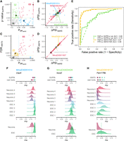
Comparison of the significance of differential AS between betAS, SUPPA, and rMATS. (A) Scatterplot comparing betAS’ and SUPPA's differential AS significance metrics. betAS’ estimated probability of differential AS, based on the proportion of differences between the beta distributed randomly emitted values per group that are >0 (Pdiff) and SUPPA's P-value, with dashed lines defining quadrants indicating the significance cutoffs considered (Pdiff > 0.95 for betAS, P-value <0.05 for SUPPA). Points are colored based on the differential AS calls by both tools: events considered differentially spliced by both betAS and SUPPA (red), by betAS (blue), or SUPPA (green) alone or by none of the tools (gray). Selected example events for each quadrant as larger outlined dots. (B) Scatterplot comparing betAS’ and SUPPA's differential AS effect size (ΔPSI). Red diagonal solid line indicates identity: ΔPSISUPPA = ΔPSIbetAS. (C) Scatterplot comparing betAS’ and rMATS' differential AS significance metrics. betAS’ Pdiff and rMATS' FDR, with dashed lines defining quadrants indicating the significance cutoffs considered (Pdiff > 0.95 for betAS, FDR < 0.05 for rMATS). Points are colored based on the differential AS calls by both tools: events considered differentially spliced by both betAS and rMATS (red), by betAS (blue), or rMATS (yellow) alone or by none of the tools (gray). Selected example events for each quadrant as larger outlined dots. (D) Scatterplot comparing betAS’ and rMATS' differential AS effect size (ΔPSI). Red diagonal solid line indicates identity: ΔPSIrMATS = ΔPSIbetAS. (E) Receiving operating characteristic (ROC) curves betAS’ differential AS calls with Pdiff (solid lines) and FPR (dashed lines), considering as ground truth the differential calls from SUPPA (yellow, P-value <0.05) or rMATS (green, FDR < 0.05). (F–H) SUPPA and vast-tools’ PSIs (top) and densities of emitted beta distributed values for individual samples (middle) and their merging per sample group (bottom, with dashed lines signing median values) for selected events illustrative of different combinations of effect size and significance of AS differences, identified by vast-tools’ IDs (VAST-DB annotation for the mouse mm10 genome assembly): (F) MmuEX0051014 (gene Usp4, chr9:108388277–108388380), (G) MmuEX0024526 (gene Isca2, chr12:84773793–84773908), (H) MmuEX0018137 (gene Fam179b, chr12:64990941–64991090). (ESCs) Embryonic stem cells.
rMATS' differential AS statistical approach relies on modeling inclusion levels by both accounting for the PSI uncertainty in individual replicates, dependent on the total number of supporting RNA-seq reads, and the (biological) variability of PSI values across replicates (Shen et al. 2014). betAS’ ΔPSI values are generally more consistent with those obtained by rMATS (Fig. 4D) than with those obtained by SUPPA2 (Fig. 4B), reflecting the consistency between vast-tools and rMATS PSI quantification. Although rMATS’ FDR is more sensitive than betAS’ Pdiff at the selected cutoff (Fig. 4C,E; Supplemental Fig. S9A–C), the significance assessment by betAS and rMATS is also more consistent than between betAS and SUPPA2. One example illustrative of the difference in sensitivity is exon MmuEX0018137 in Fam179b, whose lower inclusion in mature neurons compared to ESC (Fig. 4H) is considered significant by rMATS, but betAS Pdiff is <0.95. Visual inspection of the inclusion levels summarized with beta distributions again uncovers high interreplicate variability illustrated by the overlap of PSI distributions between ESCs and neurons, that penalizes the Pdiff (Fig. 4H), in contrast with the MmuEX0011507 exon in Clasp1, considered significantly differentially spliced between ESCs and neurons by both tools (Supplemental Fig. S9F), consistently with its known increased inclusion levels in neural tissues (https://vastdb.crg.eu/event/MmuEX0011507@mm10). Similar observations are made when choosing FPR as the significance metric for betAS (Supplemental Figs. S8C and S9C).
The comparison of differential AS between betAS and Whippet (Supplemental Fig. S10) leads to similar observations as that between betAS and rMATS.
betAS applied to differential AS between multiple groups
The differential AS approach implemented by betAS can be applied to multiple (i.e., more than two) groups in a novel ANOVA-inspired way that extends the Pdiff definition to the comparison of the differences between samples belonging to different biological conditions to those found between replicates. Statistics for multigroup differential AS are, to our knowledge, absent from the aforementioned established tools and therefore a unique feature of betAS, applicable to the study of splicing in a variety of biological contexts.
To illustrate this, we applied multiple-group betAS to the analysis of AS differences in a subset of human transcriptomes of the forebrain, hindbrain, heart, kidney, liver, and testis (Fig. 5; Cardoso-Moreira et al. 2019). By comparing the medians of differences “between” and “within” groups, both through their difference and their ratio (Fig. 5A,B), while visually inspecting their distributions (Fig. 5C–F, panels on the left), tissue-specific AS can be identified (Fig. 5C–F). While the increased number of samples renders the individual beta distributions less relevant in terms of visualization, the probability that |between|>|within| is, in this case, useful to identify AS events with differences between tissues. The selected exon HsaEX0021044 in DST, for instance, is more commonly skipped in kidney, liver, and testis, whether its inclusion is higher and more variable in brain and heart tissues (Fig. 5C). On the contrary, exon HsaEX0051256 in PTS is more excluded in brain and heart but less so in kidney, liver, and testis (Fig. 5E).
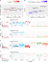
Beta distributions model inclusion level differences across multiple groups. (A) Scatterplot comparing betAS’ difference of the median of absolute differences between and within groups and the estimated probability that absolute differences between groups are greater than those within groups. Points are colored based on the estimated F-statistic as the median of absolute differences between groups divided by the median of absolute differences within groups. Highlighted points are associated with the selected example AS events in panels C–F. (B) Scatterplot comparing betAS’ difference of the median of absolute differences between and within groups and the estimated F-statistic as the median of absolute differences between groups divided by the median of absolute differences within groups. Points are colored based on the estimated probability that absolute differences between groups are greater than those within groups. Highlighted points are associated with the selected examples in panels C–F. (C–F, left) density plots of the absolute differences between (red) and within (gray), with dashed vertical lines indicative of the median values of each distribution. (Right) Beta distributions (violin plots of the emitted values) for selected events, identified by vast-tools’ IDs (VAST-DB annotation for the human hg19 genome assembly): (C) HsaEX0021044 (gene DST, chr6:56329483–56329554), (D) HsaEX0015811 (gene CLTB, chr5:175823480–175823533), (E) HsaEX0051256 (gene PTS, chr11:112100931–112100953), (F) HsaEX0055568 (gene RPS24, chr10:79799962–79799983).
In order to explore the tissue specificity of AS events or more general questions about AS differences across groups, betAS allows flagging the more variable events across groups (Fig. 5A,B), while inspection of the underlying beta distributions (Fig. 5C–F) can inform on which conditions are driving the differences. Moreover, applying the F-statistic to differential AS quantifications allows ranking events based on how robust the differences between groups are when compared to the differences between samples in the same phenotypical group (Fig. 5A,B; Supplemental Fig. S3).
betAS can also be used to study differential AS across groups with a sequential association, for example, the mouse neuronal differentiation time line data set (Fig. 6; Hubbard et al. 2013). In this case, differences between sequential groups inform on the “steps,” or the monotonicity of the variation of inclusion levels (Fig. 6A,B). Thus, “sequential” differences between groups together with their number of modes may clarify the monotonicity of transitions in inclusion levels, such as those illustrated by event MmuEX0045617 in Stxbp1, whose PSI decreases from ESC to nearly full skipping around 0 d in vitro and then progressively increases as neurons differentiate (Fig. 6C). The number of modes (or “step heights”) of the “sequential” differences and of the “generalized” differences (the median of differences found between groups in the extremes of the time line) can be useful to interpret the progression of PSI along a sequence. For instance, the inclusion of exon MmuEX0024060 in Ilf3 (Fig. 6E) decreases monotonically (from 0 until 16 d in vitro) with multiple “steps” of the same size (PSI difference), thus showing one sequential mode that is different from 0. Exon MmuEX0016666 in Elavl2 (Fig. 6F) shows a PSI increasing in the early differentiation time points (from −4 to 0 and then to 1 d in vitro), consistent with its function in safeguarding loss of neuronal ELAV function in Drosophila (Carrasco et al. 2020) with a PSI “step” that is represented by the positive sequential mode identified.
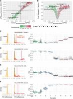
Beta distributions model inclusion level differences across sequential groups. (A) Scatterplot comparing betAS’ median “generalized” differences between groups, that is, the median of differences found between groups and the effect size (ΔPSIbetAS) between the extremes of the time line (development days 28—neurons—to −8—ESC). Points are colored based on the estimated monotonicity coefficient (see Supplemental Methods) and shaped based on the F-statistic as the median of absolute differences between groups divided by the median of absolute differences within groups. Highlighted points are associated with the selected example AS events in panels C–F. (B) Volcano plot comparing betAS’ median “generalized” differences between groups and the estimated probability that absolute differences between groups are greater than those within groups. Points are colored based on the estimated F-statistic as the median of absolute differences between groups divided by the median of absolute differences within groups. Highlighted points are associated with the selected examples in panels C–F. (C–F, left) Density plots of the PSI differences between sequential groups (orange) in the time line with rug plots (top) indicating the identified modes, with dashed vertical black line indicative of 0. (Middle) Density plots of the absolute “generalized” (red), sequential (orange), and within (gray) groups differences in PSIs, with vertical lines indicative of the median values of each distribution. (Right) Beta distributions (violin plots of the emitted values, with point indicating the mean of each distribution) for selected events, identified by vast-tools’ IDs (VAST-DB annotation for the mouse mm10 genome assembly): (C) MmuEX0045617 (gene Stxbp1, chr2:32794588–32794713), (D) MmuEX0026784 (gene Lrch2, chrX:147484754–147484804), (E) MmuEX0024060 (gene Ilf3, chr9:21388112–21388150), (F) MmuEX0016666 (gene Elavl2, chr4:91254141–91254179).
DISCUSSION
Modeling alternative sequence inclusion quantification from RNA-seq using the beta distribution allows the precision of its estimates to be proportional to the associated read coverage and reflected on the significance of differences in AS between samples. Besides the convenience of modeling precision, plotting the estimated beta distributions provides an intuitive graphical framework for understanding and evaluating the technical and biological uncertainties underlying PSI estimates. The main objective of differential AS analyses is to interpret the evidence, in terms of effect size and significance, collected for the difference in the inclusion of a given sequence of interest between biological conditions. As such, the betAS package was designed as a visual, flexible, and easy-to-use decision-support tool to assist biologists to analyze and understand their AS data.
As herein illustrated, a compromise between modeling the estimation uncertainty in the inclusion level quantification of individual samples and accounting for the variability among replicates is crucial for differential AS analysis, particularly when the sample size is small. Although several other methods using ΔPSI as a metric of the effect size have been proposed to address differential AS between conditions (Katz et al. 2010; Trincado et al. 2018), to our knowledge none has used the actual junction read counts to guide the user in visually interpreting PSI estimates and their confidence, even though these reads are proportional to the relative abundance of the alternative RNA sequences present in the profiled biological sample. betAS provides the first model that directly relies on the number of reads supporting the inclusion or exclusion of alternative sequences to provide its users with an intelligible graphical assessment of the sources of uncertainty in AS analyses. betAS facilitates the visual interpretation of the effect size and significance statistics provided by differential AS tools, currently supporting the output processed files of vast-tools (Tapial et al. 2017), rMATS (Shen et al. 2014), and Whippet (Sterne-Weiler et al. 2018), as they include inclusion and skipping read counts.
betAS’ visual approach can be particularly helpful in interpreting the uncertainty in PSI estimates of AS events supported by very few reads. These events’ beta distributions are more dispersed than those for higher read counts and the variability in the PSI estimation is passed on to the comparison between groups, reflected on the respective significance quantification, and can be visually inspected via the shape of the beta distributions. betAS thereby enables users to visually assess if the samples’ read depth is enough for profiling the AS events of interest. This is particularly relevant for RNA-seq data sets with a small sample size, a large proportion of those generated and used to study specific splicing regulatory mechanisms, in which the impact of individual samples’ read coverage on the precision of differential AS analysis is stronger. Importantly, the implementation of the betAS pipeline as a web app allows any user, irrespectively of their familiarity with R or the command line, to perform differential AS analyses across two or more conditions.
While betAS harbors useful features for AS analysis, it also has inherent limitations. Firstly, betAS relies on read count data obtained from different AS analysis tools, each dependent on a mapping approach, whose accuracy impacts the precision of inclusion/exclusion calling on which PSI quantification depends. Importantly, this dependence on prior read count data implies that users are required to have minimum computational proficiency, to run sequence alignments. We compared, for the same sample, read count estimates by vast-tools, rMATS, and Whippet, finding them overall generally (but not perfectly) consistent across tools (Supplemental Fig. S11A–C). PSI quantifications are also generally consistent but we found extremely discrepant events (e.g., PSI of 0% from one tool and of 100% from another), mostly associated with very low coverage (Supplemental Fig. S11D). Users are therefore advised to critically determine the mapping procedure that best matches their specific requirements, becoming familiar with the underlying assumptions guiding that choice, namely those associated with the aligner and the transcriptome annotation, to name a few.
One of the most challenging aspects of differential AS analysis is the assessment of the biological and phenotypical consequences of a given alteration in PSI. PSI estimates for each biological sample always reflect a sampling of the whole set of RNA molecules therein, and relative isoform expression changes have different impacts on the PSI depending on its initial value (Supplemental Fig. S12). While the intuitive visualization provided by betAS is certainly helpful, an integrated framework to easily check the known biological implications of differential AS from available databases will contribute to a clearer analysis of the biological consequences of AS alterations and a more complete usability experience for the user.
In summary, we propose betAS as an important contribution to the AS research field, since it provides sound differential splicing analysis, even of RNA-seq data sets with low read coverage and/or small sample size, while guiding researchers to biologically relevant phenomena across multiple conditions (including time series) with its easy, visual and intelligible way of interpreting statistics supporting differential AS that are not commonly intuitively explored.
MATERIALS AND METHODS
Modeling inclusion levels from RNA-seq junction reads using the beta distribution
The betAS package and web app, developed in R (version 4.1.2), enable statistical differential AS analyses, and associated visualization, from splice junction read count tables obtained from well-established AS quantification tools: vast-tools (Tapial et al. 2017), rMATS (Shen et al. 2014), and Whippet (Sterne-Weiler et al. 2018).
AS can be quantified with RNA-seq. Transcripts in a biological sample are captured and fragmented for sequencing, and the
resulting reads are mapped to a reference of annotated gene structures, including information on the set of exons, introns
and the splice junctions between these (i.e., exon–exon and exon–intron junctions) inferred for a representative set of each
gene's transcripts. An AS event is an alternative sequence, such as an exon, that is annotated as being included in some of
the gene's transcripts but not in others. In an RNA-seq sample, the fraction of mRNAs from a gene that contains a given alternative
sequence is estimated from reads that, by mapping to exon–exon or exon–intron junctions, provide evidence for the inclusion
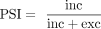
or exclusion of that sequence across the cognate gene's transcripts (Fig. 1, left). Using these reads, PSI values (Wang et al. 2008) are calculated as the ratio between the number of reads that map to the junctions defining inclusion (inc) and the sum of
these and reads that map to the junctions defining exclusion (exc) of that given alternative sequence (Fig. 1, left):
 Most AS quantification tools use PSI values alone, which do not convey information on the number of reads used in the quantification,
as the same PSI can be obtained with different levels of coverage (Fig. 1, right). Beta distributions are useful in estimating and visualizing the PSI's precision, proportional to coverage (Fig. 1, right; Supplemental Fig. S1). The beta distribution is used to model phenomena with values constrained to [0,1], namely, probabilities and proportions.
The position and shape of the beta distribution are determined by two parameters that define the distribution's mean and how
narrow the distribution is (see Supplemental Methods).
Most AS quantification tools use PSI values alone, which do not convey information on the number of reads used in the quantification,
as the same PSI can be obtained with different levels of coverage (Fig. 1, right). Beta distributions are useful in estimating and visualizing the PSI's precision, proportional to coverage (Fig. 1, right; Supplemental Fig. S1). The beta distribution is used to model phenomena with values constrained to [0,1], namely, probabilities and proportions.
The position and shape of the beta distribution are determined by two parameters that define the distribution's mean and how
narrow the distribution is (see Supplemental Methods).
In RNA-seq, coverage reflects the number of times an individual nucleotide is sequenced. Thus, when estimating PSI values, higher coverage implies higher confidence (i.e., precision) in that inclusion estimate. To model the PSI ratio and its precision for a particular AS event, the beta distribution's shape parameters can conveniently incorporate information on the number of reads used in the quantification, inc and exc, such that the mean of the distribution is directly comparable to the PSI ratio (Fig. 1), while for a given mean, the higher inc and exc are, the narrower the distribution is (Supplemental Fig. S1).
Under the aforementioned motivation and improving on previous work by others (Katz et al. 2010; Irimia et al. 2014; Shen et al. 2014; Vaquero-Garcia et al. 2016; Tapial et al. 2017), with a particular focus on the ideas underlying vast-tools’ diff module (Han et al. 2017) and Whippet (Sterne-Weiler et al. 2018), the betAS package uses beta distributions to model alternative sequence inclusion levels (i.e., PSI values) from inc and exc reads associated with annotated AS events, and their graphical representation to facilitate the interpretation of differential AS between conditions.
betAS approach for quantifying differential alternative splicing between two conditions
Estimate the effect size of splicing differences: ΔPSI
For each AS event, the modeling approach described above is used by betAS to estimate its inclusion levels per sample from the respective inc and exc read counts through the emission of random values (500 per sample by default) from a beta distribution with shape parameters inc and exc (Fig. 2A). In cases where there is deemed to be enough high-coverage replicates to probe biological variability, it may be considered appropriate to weight the number of randomly emitted values proportionally to each sample's coverage. betAS hosts this optional functionality, inactive by default. To profile differential AS between groups of samples, each AS event's inclusion level in each replicate is first modeled using a beta distribution to reflect the individual estimate's precision, proportional to the level of evidence (given by the read coverage) supporting that estimate (Fig. 2A). A joint distribution encompassing each group's replicate samples reflects both the estimation uncertainty in individual samples and the intragroup variability in PSI, therefore empirically modeling each group's PSI and its precision, while providing a statistical framework for ΔPSI (i.e., difference in PSI between groups) quantification (Fig. 2B).
Estimate the significance of splicing differences I: Pdiff
The first betAS approach to significance takes the two sets of random points per condition (Fig. 2B) and calculates, for each AS event's estimated ΔPSI, the proportion of differences between these that are greater than zero,
which has the same interpretation as asking what proportion of beta distribution-emitted values for one condition are higher
than those emitted for the other, thus reflecting the probability of differential AS, Pdiff of PSIbetas (A) being greater than PSIbetas (B) (Fig. 2C; Supplemental Fig. S2):


Estimate the significance of splicing differences II: FPR
betAS also allows the estimation of a FPR for differential AS directly from the pipeline of random number generation. Following the emission of individual beta distributions per sample and to test against the null hypothesis that there is no difference in the PSI of a given AS event between two groups (ΔPSI = 0), that is, that all PSI values in each sample of both conditions come from the same distribution, individual sample inc + exc values are used as the coverage of that event on that sample. As performed for the determination of a PSI per sample, random generation of numbers from a beta distribution is used to estimate the null distribution's PSI and its precision. Thus, shape parameters determining each sample's null beta distribution are given by random emission from a binomial distribution with number of trials, #trials = inc + exc and probability of success equal to the mean value of the PSI across all samples. This ensures that each sample's null distribution inherits the PSI precision associated with their original coverage. Then, one number is randomly selected from each of the sample's null distribution and, keeping the samples’ group assignment (i.e., which samples belong to each group), the ΔPSI between groups under the null hypothesis is calculated. The process is repeated many times (10,000 by default), and the FPR is the proportion of ΔPSI random simulations that are larger than (i.e., more extreme) or equal to the empirical ΔPSI (Fig. 2D).
Estimate the ratio of between- and within-group variabilities of PSI: F-statistic
Capitalizing on the incorporation of both the individual and group coverage-dependent PSI dispersion, betAS also enables an
ANOVA-like analysis of variance, comparing inter- and intragroup variabilities. Thus, for each event, within is considered the set of differences between each pair of samples that are part of the same group and between the set of differences between each pair of groups. The ratio of the median absolute values of between and within, therefore, provides an “F-like” statistic:
 This metric provides a compromise between the effect size of AS differences and their significance, being therefore a suitable
single metric for ranking AS events according to evidence for differential AS when both aspects are important (Fig. 2C,D; Supplemental Fig. S3).
This metric provides a compromise between the effect size of AS differences and their significance, being therefore a suitable
single metric for ranking AS events according to evidence for differential AS when both aspects are important (Fig. 2C,D; Supplemental Fig. S3).
Simulation of RNA-seq splice junction read counts from empirically derived PSI and coverage values
Simulation of empirically derived PSI and coverage values was performed following a three-step approach (Fig. 3A): First, GTEx (Lonsdale et al. 2013) transcriptomic data (version 7) were used as a source of “ground truth” tissue-specific PSIs and “real” read coverage values from which junction read counts could be simulated; second, the biological variability of tissue-specific AS events was estimated by inspecting the PSI mean and variance of events with evidence for a unimodal PSI distribution (i.e., one typical PSI mode per tissue, thus assumed as tissue-specific) and finding the variance/mean relationship of low-variance events (see Supplemental Methods); third, for the same set of representative unimodal AS events, junction read counts were simulated for a given number (N) of replicates by incorporating the biological variability estimated in step 2 and including technical variability (i.e., variation among replicates), both inspired in the “ground truth” PSIs and empirical coverages mentioned in step 1.
In detail, functions from psichomics (Saraiva-Agostinho and Barbosa-Morais 2019) were used to load sample, subject, and junction information for 563 muscle and 309 cerebellum samples (Fig. 3A, left). PSIs were quantified for 38,896 exon-skipping events using the quantifySplicing function (minReads = 0). The bimodality coefficient can be calculated based on the shape of a distribution and has been proposed as suggestive of bimodality if >5/9 (Ellison 1987). Thus, in order to select a set of exon-skipping events with tissue-specific unimodality among the 14,039 events with valid PSIs for all samples, only events with a PSI bimodality coefficient (calculated with modes R package, available as an archive at https://cran.r-project.org/src/contrib/Archive/modes) per tissue <3/9 in muscle and cerebellum were considered (Supplemental Fig. S4A).
In order to empirically estimate the minimum biological variability of real tissue-specific events (Fig. 3A, middle), the relationship between the PSI variance and mean PSI per tissue for the subset of 1143 tissue-unimodal events (Supplemental Fig. S4B–D) was assessed to identify the subset of such events that were associated with the lowest variance, that is, the tissue-unimodal events with the least observed biological noise (see Supplemental Methods).
Thus, for each tissue-unimodal AS event used as “biological inspiration,” betAS can simulate a given number (N) of replicate PSIs by the following procedure (Fig. 3A, right; Supplemental Fig. S4E; see Supplemental Methods): first, considering all samples, use the mean of the distribution of GTEx PSI values (“Original PSIs,” Supplemental Fig. S4E, top left) as the reference PSI (PSIREF) of that event per tissue and simulate, for each tissue, N PSI values from a beta distribution with shape parameters such that α + β = 138.5042 (empirically inferred, as described
in Fig. 3A; Supplemental Fig. S4D; see Supplemental Methods) and α/(α + β) = PSIREF (“Simulated PSIs,” Supplemental Fig. S4E, middle left); using the median of the GTEx coverages (covREF) associated with the original PSIs (“Original coverage,” Supplemental Fig. S4E, top right), sample N instances of cov from a Poisson distribution with λ = covREF (“Simulated coverage,” Supplemental Fig. S4E, middle right). Sampling PSI and coverage values separately ensures these likely come from different samples of the same
tissue, even though they are associated with the same event. Finally, by pairing simulated PSI and coverage values, the rbinom function is used to generate, from a binomial distribution, inc and exc read pairs per simulated replicate, to which betAS
is applied (Supplemental Fig. S4E, “betAS,” bottom left). Differences in simulated PSI values for different scenarios of N (5, 10, 50, and 100) between tissues (ΔPSI) can be obtained and compared (Fig. 3A, bottom) with respective reference differences:


betAS applied to comparisons between multiple groups
The F-statistic can inherently be used in testing differential AS between more than two groups, and the betAS pipeline extends the approach described above with that purpose. The ratio of the median absolute values between (i.e., distances between random points from samples in one group and points in the other groups) and within is again translated into the “F-like” statistic for the multiple-group comparison. Likewise, the application of the Pdiff between two groups can be extended to encompass the comparison between multiple groups (see Supplemental Methods).
Moreover, for the particular case of experimental designs with groups following a sequential relationship (e.g., time course), betAS defines sequential between as the between-group differences for any sequential pair of groups. Comparing the sign of the differences between each group and its predecessor, betAS can infer if inclusion levels are increasing or decreasing along the sequence (i.e., if there is a monotonic trend), as well as estimate a monotonicity coefficient across the complete course (see Supplemental Methods).
While there is no technical restriction on the maximum number of groups to be compared, the practical limitation lies in the visualization and interpretation of results. As the number of groups increases, interpretability becomes more challenging. Metrics can aid in prioritizing events, but visual inspection remains crucial for interpretation.
betAS visual interface
Our pipeline for differential AS analyses is accessible online at https://compbio.imm.medicina.ulisboa.pt/betAS. betAS web app was designed to guide users that are not familiar with programming in analyzing their own differential AS experiments. betAS web app can take as input a tab-delimited text file including inclusion level quantifications (PSI) together with both the inclusion and exclusion junction read counts supporting each PSI.
The app provides a launching first tab, entitled “Import inclusion levels,” that allows loading a table with AS quantifications or, by default, proceeding with an example table obtained from an RNA-seq time-series experiment on the development of seven major human organs (Cardoso-Moreira et al. 2019). At this stage, and following filtering out events with very low coverage (see Supplemental Methods), users can select the AS event types (e.g., exon skipping, intron retention, etc.) to analyze, as well as the PSI range within which to consider quantifications for analysis, while they are visually informed on the features of the population of selected events through dynamic plots and tables.
The “Group definition” tab allows users to explicitly convey the experimental design underlying their questions (sample annotation). Groups of samples can be manually generated by introducing their names, identifying their samples, and assigning colors. Alternatively, betAS can automatically screen for similarities in the samples’ names (typically the column names in the input PSI table) under the “Automatic group(s)” option, or, in the case of the default example table, use a provided feature to automatically generate groups, via the “Feature-associated group(s)” button. Groups can be deleted and created anytime by the user.
The web app supports both pairwise and multiple-group differential AS analyses. Following group definition, running differential AS analysis between groups with betAS is straightforward, involving choosing the y-axis significance metric to consider for the volcano plots and, in the case of two groups, the groups of interest for the comparison. Owing to the stochastic nature of beta distribution random number generation in betAS, each run may produce distinct outcomes. This variability poses a challenge, especially for events near significance thresholds. To address this, we introduced the option to set a seed when executing betAS, offering a practical means for reproducibility. A video tutorial on the app, to guide the user over its sections and features, is available at https://compbio.imm.medicina.ulisboa.pt/betAS/tutorial.
The betAS package, whose source code is available at https://github.com/DiseaseTranscriptomicsLab/betAS, includes functions to generate beta distributions, calculate metrics of differential AS, generate volcano plots for the global analysis of all events, as well as AS event-specific plots illustrating differential AS (such as density plots summarizing the distributions of both coverage and inclusion levels across samples).
DATA DEPOSITION
betAS web app is publicly available at https://compbio.imm.medicina.ulisboa.pt/app/betAS. Its source code is available at https://github.com/DiseaseTranscriptomicsLab/betAS.
SUPPLEMENTAL MATERIAL
Supplemental material is available for this article.
ACKNOWLEDGMENTS
We thank colleagues Manuel Irimia, Benilton Carvalho, Ramiro Magno, and all the members of the Disease Transcriptomics Lab at iMM for valuable discussions and suggestions on the manuscript. We also thank the very knowledgeable anonymous reviewers designated by RNA for their constructive and insightful suggestions and criticisms to the first version of this manuscript; their feedback greatly contributed to improved versions of both the article and betAS itself. This work was supported by the European Molecular Biology Organization (EMBO Installation Grant 3057 to N.L.B.-M.); Fundação para a Ciência e a Tecnologia (FCT Investigator Starting Grant IF/00595/2014 and CEEC Individual Assistant Researcher contract CEECIND/00436/2018 to N.L.B.-M., PhD Studentships PD/BD/128283/2017 and COVID/BD/151620/2021 to M.A.-F., UI/BD/153368/2022 to R.M.-S., and SFRH/BD/131312/2017 and COVID/BD/151928/2021 to N.S.-A., project PERSEIDS PTDC/EMS-SIS/0642/2014); and the project was cofunded by FEDER, via POR Lisboa 2020—Programa Operacional Regional de Lisboa, from PORTUGAL 2020, and by Fundação para a Ciência e a Tecnologia (LISBOA-01-0145-FEDER-007391). Funding for open access charge were provided by national funds through the FCT—Fundação para a Ciência e a Tecnologia, I.P., under the project UIDP/50005/2020 and through European Union's Horizon 2020 Research and Innovation Programme under grant RiboMed, agreement no. 857119.
Footnotes
-
Article is online at http://www.rnajournal.org/cgi/doi/10.1261/rna.079764.123.
-
Freely available online through the RNA Open Access option.
- Received July 6, 2023.
- Accepted January 15, 2024.
This article, published in RNA, is available under a Creative Commons License (Attribution-NonCommercial 4.0 International), as described at http://creativecommons.org/licenses/by-nc/4.0/.
REFERENCES
MEET THE FIRST AUTHORS


Meet the First Author(s) is an editorial feature within RNA, in which the first author(s) of research-based papers in each issue have the opportunity to introduce themselves and their work to readers of RNA and the RNA research community. Mariana Ascensão-Ferreira and Rita Martins-Silva are co-first authors of this paper, “betAS: intuitive analysis and visualization of differential alternative splicing using beta distributions.” Mariana and Rita are both PhD candidates at the Disease Transcriptomics Lab (Instituto de Medicina Molecular, Lisbon, Portugal) under the supervision of Nuno Barbosa-Morais. The Lab's research focus is on studying how alterations at the RNA level (transcription initiation, splicing, etc.) increase proneness to diseases, namely cancer, neurodegenerative disorders, and other age-related pathologies, by combining molecular and clinical information to unravel candidate therapeutic targets. Along the way, the laboratory developed tools for assisting noncomputational scientists in their analyses of transcriptomic data.
What are the major results described in your paper and how do they impact this branch of the field?
The results of transcriptomic studies, and large-scale alternative splicing quantifications in particular, can be difficult to interpret due to the high dimensionality of data and complex associated quantification metrics. We have contributed to addressing this issue by introducing an intuitive interface that facilitates both the analysis and visualization of alternative splicing quantifications and differential splicing statistics. Our tool not only offers clear visual cues but also empowers users to fully understand the involved metrics, facilitating decision-making processes that depend on their interpretation.
What led you to study RNA or this aspect of RNA science?
MA-F: I was enthusiastic about the open questions in biology and particularly fascinated by the variability of possible functions that alternative splicing confers to cells as a fine-tuner of transcriptomes.
RM-S: I became especially intrigued by the possibility of unravelling the complexities of biological processes and connecting them to diseases through the analysis of RNA variations in quantity and splicing variants.
During the course of these experiments, were there any surprising results or particular difficulties that altered your thinking and subsequent focus?
The development of betAS was a meticulous and iterative journey that originated and evolved from an internal laboratory utility. betAS evolved together with some of our collaborations, and we transformed it into a more comprehensive and universally applicable tool. This transition posed significant challenges, demanding continuous refinement and adaptation, but the journey was immensely enriching, providing valuable insights and lessons that contributed to its ultimate versatility.
What are some of the landmark moments that provoked your interest in science or your development as a scientist?
MA-F: A first landmark moment happened very early on during my PhD, as I understood how the regulation of alternative splicing contributed to the expansion of functional diversity, which was central to the design of my project. Moreover, the opportunities to present betAS to colleagues outside of the bioinformatics field often led to valuable discussions on how simplicity, cleanliness, and user-friendliness could enhance the tool. This strongly contributed to my personal commitment to clearer science communication and investment in intuitive data visualization.
RM-S: I became particularly passionate about science when I found out that we can repurpose published data sets to answer new biological questions, particularly in ageing and age-related diseases. Learning to turn raw data into effective visual communications has been a crucial part of my growth as a PhD candidate.
What are your subsequent near- or long-term career plans?
MA-F: I am still deciding on the future steps of my career, but I aspire to continue applying my data analysis skills with a focus on delivering intuitive and visual solutions to intricate problems. In studying biology or other fields, I am committed to enhancing understanding and facilitating informed decision-making through effective data representation.
RM-S: My future plans involve continuing my exploration of data science and data visualization. I aim to develop tools that enhance our understanding of the scientific process, pushing us to be knowledgeable and critical about every step of the way, and apply these resources to the study of age-related diseases.
What were the strongest aspects of your collaboration as co-first authors?
Collaborating has been an incredibly rewarding process, as our synergy enables us to achieve more collectively than each of us could independently. We are very good friends, with similar personal and scientific interests, and have learned a lot from each other by discussing the technical aspects of the tool. Rita has enabled this project to continue improving during Mariana's maternity leave, and her exceptional work ethic, along with Mariana's enduring commitment and dedication, ensured the delivery of betAS. Our collaboration has been mutually motivating, with each of us pushing the other to consistently improve and produce a complete product.