Identification of leader–trailer helices of precursor ribosomal RNA in all phyla of bacteria and archaea
- 1Interdisciplinary Biophysics Graduate Program, The Ohio State University, Columbus, Ohio 43210, USA
- 2Center for RNA Biology, The Ohio State University, Columbus, Ohio 43210, USA
- 3Department of Microbiology, The Ohio State University, Columbus, Ohio 43210, USA
- 4Department of Physics, The Ohio State University, Columbus, Ohio 43210, USA
- 5Department of Chemistry and Biochemistry, The Ohio State University, Columbus, Ohio 43210, USA
- 6Division of Hematology, Department of Internal Medicine, The Ohio State University, Columbus, Ohio 43210, USA
- Corresponding authors: fredrick.5{at}osu.edu, bundschuh.2{at}osu.edu
-
Handling editor: John Woolford
Abstract
Ribosomal RNAs are transcribed as part of larger precursor molecules. In Escherichia coli, complementary RNA segments flank each rRNA and form long leader–trailer (LT) helices, which are crucial for subunit biogenesis in the cell. A previous study of 15 representative species suggested that most but not all prokaryotes contain LT helices. Here, we use a combination of in silico folding and covariation methods to identify and characterize LT helices in 4464 bacterial and 260 archaeal organisms. Our results suggest that LT helices are present in all phyla, including Deinococcota, which had previously been suspected to lack LT helices. In very few organisms, our pipeline failed to detect LT helices for both 16S and 23S rRNA. However, a closer case-by-case look revealed that LT helices are indeed present but escaped initial detection. Over 3600 secondary structure models, many well supported by nucleotide covariation, were generated. These structures show a high degree of diversity. Yet, all exhibit extensive base-pairing between the leader and trailer strands, in line with a common and essential function.
Keywords
INTRODUCTION
The ribosome is a two-subunit, RNA-based machine responsible for protein synthesis in all living organisms. In Escherichia coli, the large (50S) subunit is composed of 23S rRNA (2904 or 2905 nt), 5S rRNA (120 nt), and 34 ribosomal proteins (RPs); and the small (30S) subunit is composed of 16S rRNA (1542 nt) and 21 RPs. Seminal work of the Nomura and Nierhaus laboratories showed that each ribosomal subunit can self-assemble in vitro, indicating that the process of subunit assembly is fundamentally a function of the rRNA and RP components themselves (Traub and Nomura 1968; Mizushima and Nomura 1970; Nomura and Erdmann 1970; Nierhaus and Dohme 1974). However, in vitro self-assembly is slow and requires nonphysiological conditions, such as high temperature and high Mg2+ concentration. In the cell, assembly of ribosomes begins cotranscriptionally and involves cis-acting pre-rRNA elements and various trans-acting assembly factors (AFs), including RNA-binding proteins, modification enzymes, helicases, chaperones, and GTPases (for review, see Davis and Williamson 2017; Gibbs and Fredrick 2018; Naganathan and Culver 2022). These AFs are believed to speed up assembly, protect premature subunits from degradation, and prevent premature subunits from entering the translationally active pool.
Ribosomal RNAs are transcribed as part of long precursor molecules. In E. coli, 16S rRNA, 1-2 tRNA, 23S rRNA, and 5S rRNA are cotranscribed from seven distinct operons (Maeda et al. 2015). Flanking each rRNA are complementary sequences, which form extended leader–trailer helices (Young and Steitz 1978; Brosius et al. 1981). These long LT helices are recognized and cleaved by RNase III, a double-stranded RNA endonuclease, yielding smaller precursors that are further trimmed by other RNases at later stages of subunit biogenesis (for review, see Deutscher 2003; Bechhofer and Deutscher 2019). Notably, the LT helices also play a more crucial role in subunit biogenesis, independent of RNase III (Liiv and Remme 1998; Warner et al. 2023). Experiments in which the LT helix of 16S rRNA is progressively shortened show that at least 17 bp are needed to form active subunits in either wild type or Δrnc (RNase III) E. coli cells (Warner et al. 2023). Expression of the mature (fully trimmed) 16S rRNA in cells (with the help of an engineered promoter and hammerhead ribozyme) gives no active subunits (Warner et al. 2023). The fact that 30S biogenesis in the cell depends so strictly on the LT helix came as a surprise, because mature 16S rRNA supports efficient subunit assembly in the test tube.
Why LT helices are required to make ribosomal subunits in vivo but not in vitro remains unclear. We have hypothesized that formation of an LT helix enables subunit assembly to be thermodynamically favorable in the cell (Warner et al. 2023). By bringing together the 5′ and 3′ ends of pre-rRNA, the LT helix may limit the number of conformations the pre-rRNA can adopt, counteracting cellular drivers of RNA unfolding and promoting productive paths of assembly. Indeed, a growing body of evidence indicates that RNA molecules tend to be less structured in vivo than in vitro, due at least in part to enzymes like helicases that hydrolyze ATP (Rouskin et al. 2014; Mustoe et al. 2018; Ganser et al. 2019; Jarmoskaite et al. 2019; Xiang et al. 2023; Aseev et al. 2024). Mutational analysis has shown that the function of the 16S LT helix depends on its structure rather than its sequence (Warner et al. 2023), in line with our hypothesis.
If LT helices play such a fundamental role, one would expect them to be universal. Saito et al. (2000) used a computational approach to screen 12 bacterial and three archaeal species for the presence of 16S and 23S LT stems. In brief, the approach involved computational hybridization of each of various 50 nt segments of the leader across the trailer region, and vice versa. They found compelling evidence for LT stems in most but not all of their species. One organism, Deinococcus radiodurans, appeared to lack LT helices for both 16S and 23S rRNA. However, given that there are many ways to generate a folded RNA involving two segments (i.e., the leader and trailer regions) and that 15 species cannot capture the full diversity of prokaryotic life, the questions of whether LT helices/structures were missed or are truly absent and if LT helices are truly universal remain open.
In this work, we use two approaches to investigate the prevalence of LT stems/structures in pre-16S and pre-23S rRNAs. First, we compare the folding of native LT versus random-shuffled LT sequences and deduce the degree of pairing between leader and trailer strands. Second, we look for nucleotide covariation, a reliable predictor of functional RNA helices (Gutell 2014), among related LT sequences to identify and define LT structures. Based on analysis of 35,948 LT sequences from 4724 organisms, we find that LT stems are ubiquitous across all tested phyla of bacteria and archaea.
RESULTS
Shuffling identifies LT stems of 16S rRNA
As a first approach to exhaustively screen LT sequences across whole phyla for the presence of a stem, we developed the shuffling method, an overview of which can be found in Figure 1A. We use computationally predicted RNA structures of LT sequences (Fig. 1B) and quantify their “stemness”; i.e., how strong an LT helix stem is in a structure, by counting the number of 10 nt sliding windows (SWs) along each strand that contains an SW on the opposite strand with at least 8 LT bps, defined as the number of successful sliding windows (SSWs) (Fig. 1C). This approach enables flexibility for the method to handle small bulges in an LT helix which we assume do not preclude stem formation. Since in reality a multitude of possible structures can form from a given sequence, we do not solely use the minimum free energy (MFE) structure, but sample 100 plausible structures from the partition function and take the average of the stemness measure over these 100 structures. This average number of SSWs alone does not provide an answer for what threshold is to be considered a “strong” or “weak” stem, and establishing such a general threshold is impossible due to confounders such as GC content and variable LT sequence length. To address this, we apply LT sequence shuffling that exactly preserves dinucleotide frequencies to generate 100 shuffled LT sequences for each biological one. The same structure prediction and SSW counting is applied to the shuffled sequences (i.e., the average number of SSWs from its 100 structures is compiled for each shuffled sequence) to obtain a random background distribution to which the biological signal can be compared to calculate a z-score, which has an easily explainable meaning across species (i.e., how many shuffled standard deviations above the shuffled mean is the biological signal).
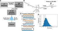
A shuffling method identifies LT helices of 16S rRNA. (A) For each LT sequence, dinucleotide frequency preserved shuffling was applied 100 times, generating 101 total sequences. For each sequence, the ViennaRNA package was used to sample 100 secondary structures. For each of the 10,100 generated structures, an SW matching approach was applied to determine the LT stem signal, which was averaged over the 100 structures sampled for each sequence to obtain the sequence's stem signal. The average biological sequence signal was compared to the mean and standard deviation of the shuffled sequence signal distribution to determine the z-score, representing the relative strength of an LT stem forming in the biological sequences against a random background. (B) An example biological LT structure of 16S rRNA of E. coli, where the sequence corresponding to the mature rRNA has been replaced by NNNNNNNNNN (C) (i) a successful LT SW, with 10 of 10 positions containing an LT bp, (ii) an unsuccessful LT SW, where only seven of 10 positions contain an LT bp, (iii) a successful LT SW, where nine of 10 positions contain an LT bp. (D) The distribution of z-scores for all 17,942 16S LT sequences, where black dotted lines are drawn at z-scores of 0, 1, and 2; used to classify evidence for LT stems as absent, weak, intermediate, and strong.
Figure 1D shows the distribution of all 16S z-scores across bacteria and archaea. The vast majority of LTs exhibit z-scores above 0, signifying that the biological sequence contains a stronger stem signal than the shuffled sequence distribution, with median 2.83 for all LTs. Black dotted lines are drawn at z-scores of 0, 1, and 2 to visually separate absent, weak, intermediate, and strong evidence of an LT stem as determined by this method. We chose a z-score of 2 as a threshold for strong evidence of an LT stem because it corresponds to a P-value of 0.05. As a control, we chose random sequences for 2000 16S cases and 2000 23S cases and reran the shuffling method, producing distributions where only 4.50% and 4.25% of the z-scores are above 2, respectively (Supplemental Material A).
Covariation and consensus structures identify LT stems of 16S
A challenge with the shuffling method is determining the right leader and trailer sequence boundaries (i.e., upstream and downstream of the rRNA annotation). Incorrect gene annotations could result in the leader or trailer sequences not being long enough to capture the LT stem. To address this challenge, and inspired by our previously conducted work identifying 16S LT stems across members of the Enterobacteriaceae family (Warner et al. 2023), we developed the covariation method, summarized in Figure 2A. This approach gathers 500 nts of the leader and 300 nts of the trailer (ignoring gene annotations) and then clusters the LT sequences by both their taxonomic class and sequence similarity. We then leverage consensus structure prediction from many related LT sequences using the RNAClust tool (an example structure is shown in Fig. 2B, and all structures are available at 10.5281/zenodo.11051088). RNAClust builds consensus structures by examining both primary sequence alignments and RNA folding sequence-structure alignments using LocARNA to construct a hierarchical tree (Will et al. 2007, 2012; Raden et al. 2018). Base pairs in a consensus structure are identified through pairs of locations that show different nucleotides in different sequences while preserving their ability to pair. Covariation describes the number of unique combinations of nucleotides in the base pair across all sequences. Within the consensus structures, base pairs are colored by their covariation and tinted by mismatch rate. Consensus structures form large loops and contain lightly shaded (i.e., weakly supported) base pairs in regions that are not well conserved, causing these divergent regions to remain largely unstructured in the consensus structure (Fig. 2B, upper left portion). These divergent regions tend to appear far away from the mature rRNA. This aspect of consensus structures eliminates worry about gathering too many nucleotides, since they will very likely all belong to divergent regions and thus will not falsely contribute to signals for an LT stem. We measure the “stemness” of all members contributing to a consensus structure by applying the same SSW-method as the shuffling method and by quantifying the fraction of LT bps that exhibit covariation (i.e., are not shaded red in the consensus structure). The example shown in Figure 2B demonstrates an LT stem that exhibits good covariation support in addition to producing SSWs that meet the method criteria.
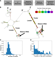
Analysis of covariation in LT helices of 16S rRNA. (A) Each taxonomic class was analyzed independently. The LT sequences from species belonging to the class were compiled. Sequences sharing sequence similarity were clustered together using the MMSeqs easy-cluster function to reduce RNAClust computational burden and to generate realistic consensus structures. For each sequence cluster, RNAClust was run to determine the consensus structure and its covariation. The same SSW approach as for the shuffling method was applied. The fraction of LT bps exhibiting covariation (e.g., non-red colored bps) was computed. (B) The RNAClust consensus structure rooted at Staphylococcus piscifermentans. The consensus structure creates large loops where structure is not conserved, typically far away from the LT stem and mature rRNA (upper left area). Color-coding indicates the number of different base pairs observed at a given position: red, 1; yellow, 2; green, 3; cyan, 4; blue, 5; magenta, 6. Tint level reflects the fraction of mismatches (full color indicating no mismatches, followed by a lighter tint up to 10% mismatches, even lighter for up to 20% mismatches, and no coloring for above 20% mismatches). (C) The distribution of all SSW scores, where the black dotted line corresponds to the threshold used to distinguish LT sequences with evidence for a stem from LT sequences without such evidence. (D) Histogram showing the degree of covariation across all structures, where the black dotted line corresponds to the threshold that distinguishes weak from strong covariation.
Figure 2C shows the distribution of SSWs for all 16S LT sequences across bacteria and archaea. The black dotted line at a number of SSW value of 15 corresponds to the threshold we used to distinguish consensus structures with evidence of an LT stem from those without such evidence (our rationale for choosing 15 as a threshold is described in Supplemental Material B). The majority of LTs in this method exhibit a stem. We note that consensus structure prediction with RNAClust is computationally expensive, preventing us from generating shuffled sequences and computing a z-score.
Figure 2D shows the distribution of LT covariation fractions, where the black dotted line at fraction covariation of 0.25 is the threshold that we chose to distinguish weak from strong covariation. Fifty-six percent of LTs have structures that are not well supported by covariation, due to paucity of sequence data for those clades of the taxonomy tree.
While the covariation method is a powerful tool, it might not produce a prediction for all LTs. This may be because (1) the full leader or trailer regions are not contained within the gathered genome sequence segments or (2) the sequence similarity clustering conducted before running RNAClust produces a sequence cluster of size one (i.e., no closely related LT sequences in the same taxonomic class). We find that of the 18,040 16S rRNA LTs, the covariation method makes a prediction for 15,984 (88.6%) and predicts an LT helix for 15,512 (97.6% of the ones it makes a prediction for).
Combination of methods reveals broad prevalence of LT stems
The shuffling method and the covariation method each carry their own strengths and weaknesses. An LT with no stem prediction in either method could be due to an approach or technical issue and yet still contain a stem. For example, in the shuffling method, an upstream or downstream gene annotation could prevent enough nucleotides from being gathered; in the covariation method, LT sequences of too much dissimilarity could be brought together. On the other hand, it is unlikely that an LT with a stem prediction actually contains no stem, especially when the predicted LT stem is supported by covariation. In the shuffling method, this argument is supported by the fact that many of observed z-scores are much higher than 1, the threshold we used to call an LT stem (see Fig. 1). In the covariation method, we used an SSW threshold of 15, and again many of the LTs are much higher than this threshold (see Fig. 2). With these considerations in mind, we reason that the most likely failure mode of either method is a false negative. Therefore, we use the combined prediction from both methods and assume that an LT with a predicted stem in either method indicates the true presence of an LT stem. Figure 3A and B shows phylogenetic trees rooted at the proteobacteria phylum. The leaves in the Figure 3A tree are shaded by the shuffling method's z-score and in the Figure 3B tree by the covariation method's number of SSWs and LT covariation fraction. In both trees, blue leaves represent weak stems (i.e., lower z-scores and number of SSWs), and red leaves represent strong stems (i.e., higher z-scores and number of SSWs). Gray leaves represent an LT with no prediction for that method (but a prediction in the other method). Collectively, the trees indicate that LT stems are ubiquitous in proteobacteria.
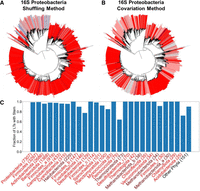
Identification of 16S LT helices across all phlya. (A,B) A phylogenetic tree of Proteobacteria, with leaf nodes colored based on shuffling-method z-scores (A; dark blue: no signal, light blue: weak signal, light red: intermediate signal, dark red: strong signal, see Fig. 1) or covariation-method results (B; dark blue: no evidence for stem with strong covariation, light blue: no evidence for stem with weak covariation, light red: evidence for stem with weak covariation, dark red: evidence for stem with strong covariation, see Fig. 2C,D). Gray leaf nodes signify no prediction. (C) The fraction of LT sequences from each phylum with an LT stem, predicted by either method (shuffling z-score ≥ 1 or covariation number of SSWs ≥ 15). Bacterial phyla, red labels; archaeal phyla, brown labels. Phyla with <25 LT sequences were grouped together in other phyla. The number of LTs for each phylum are noted in parentheses.
We further leverage the practice of using the two methods to complement each other in Figure 3C, which shows the fraction of all LTs in every phylum where at least one method predicts an LT stem. Bacterial phyla names are shaded red and archaea are shaded brown. Nearly all phyla have a high fraction of LTs with a predicted stem in either method, with only Fusobacteriota, Deinococcota, and Actinobacteriota containing a fraction <0.8.
LT stems of 23S rRNA are ubiquitous
Next, we applied both the shuffling and covariation method to 23S LTs. Consistent with the 16S data described above, a large fraction of bacteria and archaea were identified as containing LT stems. Each method's measurable signals for 23S are shown in Figure 4. Of 17,908 23S rRNA LTs, the covariation method makes a prediction for 14,964 (83.6%) and predicts an LT helix for 14,047 (93.9% of the ones it makes a prediction for).
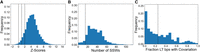
Identification of LT helices of 23S rRNA by both methods. (A) The distribution of all shuffling method z-scores. Black dotted lines are drawn at z-scores of 0, 1, and 2 used to classify evidence for LT stems as absent, weak, intermediate, and strong. (B) The distribution of all covariation method SSW scores. The black dotted line corresponds to the threshold used to distinguish LT sequences with evidence for a stem from LT sequences without such evidence. (C) Histogram showing the degree of covariation across all structures, where the black dotted line corresponds to the threshold that distinguishes weak from strong covariation.
The same set of proteobacteria trees as in Figure 3 for 16S are shown in Figure 5 for 23S. Similar to 16S, the two 23S trees visually complement each other, where if one method exhibits a weak stem prediction the other exhibits a strong stem prediction in any clade of the tree. We thus conclude that 23S LT stems are also ubiquitous in proteobacteria. Figure 5C shows the fraction of all 23S LTs in every phylum where at least one method predicts an LT stem. As with 16S, nearly all phyla have a high fraction of LTs with a predicted stem by either method; only Spirochaetota and Deinococcota contain a fraction <0.8. Phylogenetic trees showing the prevalence of 16S and 23S LT helices across each phylum are shown in Supplemental Material C.
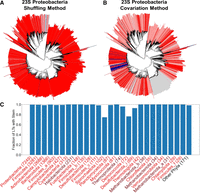
Identification of 23S LT helices across all phlya. (A,B) A phylogenetic tree of Proteobacteria, with leaf nodes colored based on shuffling-method z-scores (A; dark blue: no signal, light blue: weak signal, light red: intermediate signal, dark red: strong signal, see Fig. 1) or covariation-method results (B; dark blue: no evidence for stem with strong covariation, light blue: no evidence for stem with weak covariation, light red: evidence for stem with weak covariation, dark red: evidence for stem with strong covariation, see Fig. 2C,D). Gray leaf nodes signify no prediction. (C) The fraction of LT sequences from each phylum with an LT stem, predicted by either method (shuffling z-score ≥ 1 or covariation number of SSWs ≥ 15). Bacterial phyla, red labels; archaeal phyla, brown labels. Phyla with less than 25 LT sequences were grouped together in other phyla. The number of LTs for each phylum are noted in parentheses.
Species without an LT stem prediction are likely false negatives
Inspection of the trees revealed a small number of LTs where neither method provided evidence of a stem. One such example is Geobacillus subterraneus 16S, whose location in a zoomed-in clade of Firmicutes is shown in Figure 6A. Figure 6B shows the G. subterraneus consensus structure from the covariation method, where one long leader–leader helix (labeled “L”) and two long trailer–trailer helices (labeled “T1” and “T2”) are seen.
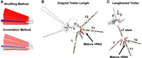
False negatives due to missing sequence data. (A) A branch of the 16S Firmicutes tree containing Geobacillus subterraneus LTs, shaded blue (indicating no evidence for a stem) by both methods. (B) The RNAClust consensus structure, where no LT stem is observed. Labels T1 and T2 denote trailer–trailer helices, and L denotes a leader–leader helix. (C) The RNAClust consensus structure with an adjusted trailer length of 500 nts, where an LT stem is observed. The same numbering schema denotes helices between (B) and (C). The increased trailer length captures the LT stem, indicating that an LT stem exists in G. subterraneus, and that both the shuffling method (for which even fewer trailer nucleotides are gathered due to a downstream gene annotation) and the covariation method under default settings simply do not gather enough trailer nucleotides for this species. Full-page figures for each structure in (B) and (C) are available in Supplemental Material D.
We noted that these two large trailer–trailer helices, which are well supported by covariation, account for much of the 300 nt trailer sequence analyzed and hypothesized that the trailer strand of the LT helix lies further downstream. Figure 6C shows the G. subterraneus consensus structure with an elongated trailer (adding 200 nts to the default trailer length). Indeed, in addition to the leader (L) and trailer (T1 and T2) helices, a clear LT stem is now observed. Thus, we conclude that G. subterraneus 16S contains LT stems, and both methods with default settings fail to predict an LT stem due to the abnormally large trailer–trailer helices causing not enough trailer nucleotides to be acquired.
A closer look at those cases with no initially predicted LT stem revealed that virtually all LTs indeed contained a stem. Both methods failed to detect the stem due to insufficient trailer length or internal bulges or loops disrupting continuous runs of LT SSWs (see Supplemental Material E, which describes repeating both methods with an extended trailer region and identifies additional LTs). We extended this analysis to consider all LTs within a species and found that most LTs with no predicted stem in either method are from a species containing another LT with a predicted stem (see Supplemental Material F).
Deinococcota show weak LT stems
Saito et al. (2000) screened 15 species of bacteria and archaea for the presence of 16S and 23S LT stems, using an “annealing” approach in which pairing free energies of segments of the leader and segments of the trailer were systematically determined. They found evidence for LT stems in many species but no evidence for LT stems flanking either 16S or 23S rRNA in D. radiodurans. We found relatively low fractions of LTs in the Deinococcota phylum (16S: Fig. 3C, 23S: Fig. 5C). Figure 7A and B show the phylogenetic tree rooted at Deinococci, with the same leaf shading schema described previously, where D. radiodurans is tagged with a black arcing line. In 16S, both methods identify weak D. radiodurans stems; however, examination of the consensus structures (Fig. 7C) clearly shows the presence of an LT stem (albeit, weakened by bulges and internal loops). In 23S, both methods predict an LT stem for two of the three rRNA copies, the consensus structure of which is shown in Figure 7D (the other rRNA copy did not result in a prediction). We conclude that D. radiodurans contains LT stems for both 16S and 23S rRNA, although these stems appear weaker than those of other species.
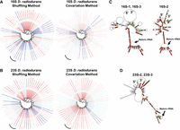
Analysis of LT helices in the Deinococcota. Deinococcota trees and RNAClust Deinococcus radiodurans consensus structures in both 16S (A) and (C) and 23S (B) and (D). The position of D. radioduran's 3 LT sequences on the trees (A and B) is indicated by a black arcing line. In both 16S and 23S, the consensus structures show an LT stem, albeit a weak one. Full-page figures for each structure in (C) and (D) are available in Supplemental Material D.
DISCUSSION
While we (Warner et al. 2023) and others (Saito et al. 2000; Shi et al. 2011) have previously screened a limited number of species for the presence of LT helices, to our knowledge no study to date has comprehensively analyzed all known bacteria and archaea to assess the presence of 16S and 23S LT helices until this one. The results of this study provide strong evidence that LT helices are ubiquitous in both 16S and 23S across all known prokaryotes through two computational methods. Nearly all (97.5% of 16S and 98.4% of 23S) rRNAs contained an LT helix with default method parameters, and additional analysis concluded that virtually all of the remaining rRNA contained an LT helix but evaded our methods due to lengthened trailer–trailer helices or internal loops/bulges (Supplemental Materials E and F). Our findings suggest that LT helices serve an important and common purpose across the prokaryotes. Work in E. coli has shown that LT helices of both 16S and 23S rRNA are crucial for formation of active subunits (Liiv and Remme 1998; Warner et al. 2023), and it will be worthwhile to experimentally determine the contribution of LT helices to subunit biogenesis in organisms of other phyla in the future.
Previously, Saito et al. (2000) screened 12 bacterial and three archaeal genomes for the presence of 16S and 23S LT stems and concluded that most genomes contained LT stems with the notable exception of D. radiodurans. Our methods identify clear evidence of LT stems in D. radiodurans (Fig. 7), with several regions supported by covariation. We hypothesize that the “annealing”-based method conducted by Saito et al. effectively missed intermittent bulges and loops occurring along the length of the LT helix, features that our dual-method approach can more robustly take into account. Notably, biochemical studies (Chen et al. 2007) of 23S maturation in D. radiodurans have provided evidence for an LT helix, with a similar pattern of bulges as that of Figure 7D. Deinococcus radiodurans and related organisms naturally lack RNase III and instead rely on other endonucleases to facilitate rRNA processing. It is possible that evolutionary loss of RNase III in these organisms is a consequence of bulge-laden LT helices, which RNase III fails to recognize (Lejars et al. 2021). As noted previously (Saito et al. 2000), archaea also lack RNase III yet contain LT helices, consistent with an important role for LT helices independent of RNase III.
Both methods that are introduced in this study have limitations. Internal loops and bulges are naturally present in many of the LT helices, and accounting for these structural features with a scoring mechanism is challenging. We used a sliding-window-based approach to quantify LT stem signal; however, the method is not perfect and can predict false negatives for LTs with shorter stems that contain bulges or loops. We note that quantitative thresholds are used in this sliding-window-based metric (e.g., 8 LT bps within a 10 nt SW), and these thresholds are somewhat arbitrary. We evaluated several combinations of thresholds (data not shown) and determined that our choice of 8 in 10 was a reasonable one. We also note that both methods are more likely to produce false negatives than false positives. In the case of the shuffling method, we use a z-score to capture confounding factors about each individual LT sequence by measuring the relative stem signal of biological structures versus randomly scrambled sequence structures. While a high z-score could theoretically be achieved with a weak biological LT stem but no shuffled LT stems, we argue that this scenario is highly unlikely, especially since we generate 100 shuffled sequences per biological sequence. We use a z-score cutoff of 1 to signify a predicted LT stem, and note that this carries a statistical meaning (i.e., there is only a 16% chance for false positives). We note that the majority of observed z-scores are much higher than 1 (see Figs. 1 and 4). Whereas for the covariation method, we observe consensus structures directly and use a threshold of 15 from the SW metric as a cutoff for whether the stem is biologically relevant. The threshold of 15 corresponds to an observed z-score of 1 (see Supplemental Material B). Additionally, the majority of observed number of SSWs was well above 15 (see Figs. 2 and 4). We argue that the principle in which both methods are more likely to produce false negatives than false positives is a reasonable assumption, and thus apply it in Figures 3 and 5 to observe the distribution of LT helices across prokaryotic phyla.
In our previous work (Warner et al. 2023), we identified some Enterobacteriaceae species that contain rRNA operons with unrelated 16S LT structures. Providencia heimbachae, for example, contains seven operons encoding virtually identical 16S rRNA, but the flanking RNA folds into one of two clearly distinct structures (termed Providencia I and Providencia II), depending on the operon. In this current work, we similarly observe cases in which different types of LT structures, which can include variable leader–leader and/or trailer–trailer helices, occur within the same species. One example is Bacillus subtilis, which contains 10 rrn operons that encode five unique 16S LT structures, each with distinct structural features but all containing an elongated LT helix (Supplemental Material G). While sequence heterogeneity among these operons has been appreciated for some time (Shaver et al. 2001, 2002), the corresponding RNA structures have until now been unclear. Interestingly, a significant subset of organisms contains as many unique LT structures as they have operons (see diagonal signals in Fig. S14 from Supplemental Material H), raising the possibility of differential (operon-dependent) regulation of subunit biogenesis in these organisms. While these observations are intriguing and should inspire future research, variable features cannot speak to the primary function of LT structures. Common to these diverse LT structures is that they bring together the 5′ and 3′ ends of rRNA, which most likely holds relevance to their key role.
Subunit assembly begins as soon as the nascent pre-rRNA transcript emerges from RNA polymerase. However, key events in the process must occur posttranscriptionally (i.e., after transcription of the trailer), because no active subunits are generated without the LT helix (Liiv and Remme 1998; Warner et al. 2023). What critical role does the LT helix play? We propose that formation of the LT helix promotes late-stage assembly (Warner et al. 2023). By bringing the 5′ and 3′ ends of rRNA together, the LT helix would limit the conformational dynamics of pre-rRNA and counteract helicases and other drivers of RNA unfolding. Domains/blocks of the subunit formed cotranscriptionally would be oriented upon LT helix formation, which may facilitate further folding events and rearrangements needed to finish subunit assembly. Another nonmutually exclusive possibility is that the LT helix protects premature particles from degradation. Robust quality-control mechanisms that govern ribosome turnover exist in the cell, and signals that distinguish target versus nontarget particles remain incompletely understood (Cheng and Deutscher 2003; Connolly and Culver 2013; Maiväli et al. 2013; Jain 2018; Sharma and Woodson 2020). Certainly, further work will be needed to clarify why LT helices are so critical for ribosome biogenesis.
Our previous (Warner et al. 2023) and current findings suggest that LT helices play a fundamental role in ribosome biogenesis. Yet, pre-rRNAs of eukaryotes lack LT helices. How can this apparent conundrum be explained? The process of ribosome assembly in eukaryotic cells is complex (Ebersberger et al. 2014; Klinge and Woolford 2019; Hurt et al. 2023, 2024). It involves >200 nonribosomal factors (proteins, protein complexes, and small nucleolar RNPs) and the trafficking of assembly intermediates from the nucleus to the cytoplasm. Cryo-EM structures of various intermediates, representing different stages of 40S and 60S assembly, have been determined (Wu et al. 2016; Barandun et al. 2017; Cheng et al. 2017; Kater et al. 2017; Sanghai et al. 2018). Each of these intermediates contains many tightly bound AFs, which interact with one another, creating a structural scaffold for pre-rRNA. We envisage that these factor-based scaffolds facilitate rRNA folding by constraining pre-rRNA dynamics, functionally substituting for LT helices. Compelling new evidence suggests that eukaryotes evolved from archaea (Zaremba-Niedzwiedzka et al. 2017; Eme et al. 2023), and LT helices are ubiquitous in the extant archaea (Figs. 3 and 5). As early eukaryotes evolved, LT helices were probably lost after the factor-based scaffolds arose.
MATERIALS AND METHODS
Selection of genomes and rRNA annotation
A list of bacteria and archaea designated as “species representative” and with an NCBI assembly level “complete genome” was obtained from the Genome Taxonomy Database (GTDB) (Parks et al. 2020) bacteria v120 and archaea v53_r207. Genomes and annotations were obtained from NCBI using the RefSeq assembly summary file available on NCBI's file transfer protocol system. In total, 4724 such organisms were identified (Supplemental Material). For each organism, barrnap v0.9 (Seemann 2013) was used with default settings to predict 16S and 23S rRNA sequences.
Shuffling method for identification of leader–trailer stems
Identification of leader–trailer (LT) regions
For each complete 16S and 23S pre-rRNA annotation (henceforth referred to only as 16S and 23S rRNA), leader and trailer sequences were extracted upstream and downstream from the rRNA, respectively, taking into account strand direction. For 16S rRNA, the leader sequence was defined as the region from the nearest upstream gene (or end of the genome contig) to the 5′ end of the rRNA, or the 500 nts upstream of the rRNA, whichever was smaller, plus the first 15 nts of the barrnap annotated rRNA (corresponding to helix h0 in E. coli [Warner et al. 2023]). The trailer sequence was defined as the region from 2 nts outside the barrnap annotated rRNA (corresponding to the mature 3′ end in E. coli) to the next downstream gene annotation (or end of the genome contig), or the 300 nt downstream from the rRNA, whichever was smaller. The LT sequences were defined similarly for 23S rRNA, except the leader sequence and trailer sequence boundaries were defined as the first nucleotide outside the barrnap annotated rRNA and the first nucleotide inside the barrnap annotated rRNA, respectively, excluding H1 from the 23S leader–trailer sequences. Gene annotations were derived from the genome's GFF file. Sequences for which the leader or trailer sequence length was <40 nts were discarded from the analysis. For 16S and 23S, 17,942 and 17,770 LT sequences were available, respectively.
Application of dinucleotide-conserved shuffling
For each LT sequence pair, the leader and trailer sequences were independently shuffled 100 times each using the fasta-dinucleotide-shuffle program from the MEME Suite (Bailey et al. 2015). This program implements the Altschul-Erickson algorithm (Altschul and Erickson 1985), which shuffles the nucleotides while exactly preserving dinucleotide frequencies.
Generation of RNA secondary structures
Each LT sequence pair (1 biological and 100 shuffled, e.g., 101 total sequences per original LT pair) was concatenated with a string of NNNNNNNNNN in between the leader and trailer sequences to represent the position of the mature rRNA. The ViennaRNA software suite (Hofacker et al. 1994; Lorenz et al. 2011) was used to generate the folding landscape of plausible RNA secondary structures supported by the sequence. One hundred structures were sampled from the partition function using the “pbacktrack” function, in total generating 101 × 100 = 10,100 structures per original LT sequence.
Quantification of LT stem signal
For each LT structure, an SW of size 10 nts was independently applied to the leader and trailer sequence positions. For each
10 nt SW, all possible 10 nt SWs of the opposite strand were examined (e.g., if the original SW was on the leader, all trailer
SWs were interrogated) to determine if for at least one SW on the opposite strand, at least 8 nts of the SW on the original
strand formed an LT base pair (bp) with a nucleotide in the SW on the opposite strand. The total number of SWs passing the
above condition, designated the number of SSWs, was compiled for structures originating from the biological sequence and all
shuffled sequences. The number of SSWs was averaged over all 100 sampled structures for a given sequence. This mean number
of SSWs for each of the 100 shuffled sequences together represented a distribution, from which the mean (μshuffled) and standard deviation (σshuffled) were computed with the Python SciPy package (Virtanen et al. 2020). The SSW threshold of 8 bps in a 10 nt SW were chosen from several other analyzed thresholds (data not shown) as a reasonable
tradeoff between a stringent bp requirement and tolerance for minor bulges. The z-score of the mean number of SSWs from the biological sequence (μbiological) versus the scrambled mean number of SSWs distribution was computed to quantify how strongly an LT stem formed in the biological
sequence (compared to the background of randomly shuffled sequences, which accounts for confounding factors such as GC content)
via the following equation.

Covariation method for identification of leader–trailer stems
Identification of leader–trailer regions
For each complete 16S and 23S rRNA annotation, LT sequences were extracted in a similar manner to the shuffling method except that 500 nts upstream and 300 nts downstream from the barrnap, annotated rRNA defined the leader and trailer boundaries, respectively (e.g., gene annotations were ignored). The 500 and 300 nts thresholds were chosen as conservative thresholds that were longer than the distance to the nearest gene from nearly all 16S and 23S rRNA leader–trailers (data not shown), yet avoided excessive computational runtimes and spurious non-LT helix predictions. Annotations for which 500 and 300 nts were not available upstream and downstream (respectively) of the rRNA were discarded. LT sequences were concatenated with the 10 joiner N's, representing the mature rRNA. For 16S and 23S, 15,102 and 14,964 LT sequences were available, respectively.
Sequence similarity clustering
To reduce computational burden, sequences were preclustered by taxonomy and sequence similarity before running covariation structure predictions. First, LT sequences were grouped by their GTDB taxonomic class. Second, sequences were clustered together in each class using the “easy-cluster” function from the MEME suite (Bailey et al. 2015) (settings ‐‐min-seq-id 0.3 -c 0.5 ‐‐cov-mode 1).
Covariation structural modeling
The sequences in each cluster were deduplicated and the RNAClust tool was run with the RNASoup flag enabled, and structural constraints preventing the joiner N's from base-pairing. Clusters with only a single sequence were ignored. The RNAClust tool was altered such that the nucleotide tint level in the consensus structure corresponds to the fraction of mismatches at each position (full color indicating no mismatches, followed by a lighter tint up to 10% mismatches, even lighter for up to 20% mismatches, and no coloring for above 20% mismatches), rather than the number of mismatches that the RNAClust program uses by default. Additionally, the joiner N's were represented in the RNAClust consensus structure images by the “#” character instead of the default “−”.
Measurement of LT stem signal
The RNAClust consensus structure for each sequence cluster was analyzed for both stem signal and level of covariation evidence supporting the structure. To determine the stem signal, the same SSW-based approach as the shuffling method was used. To determine the level of covariation evidence, the fraction of all LT bps that exhibited any nonzero degree of covariation (i.e., were not colored red in the consensus structure) was computed.
Results from the shuffling method and covariation method for every analyzed species and operon are detailed in the Supplemental Tables.
Annotation of phylogenetic trees
Phylogenetic trees were generated using the GTDB taxonomy system (Parks et al. 2020) and iTOL (Letunic and Bork 2021). GTDB taxonomic tree distances (i.e., branches) between each node were maintained. Species leaf nodes were split into the number of complete rRNA annotations available and joined together by a branch of length 0 to represent all analyzed LT structures in a single tree. Separate phylogenetic trees were created for each taxonomic phylum; for the covariation method, which preclusters species by taxonomic class, all classes were joined in their respective phylum.
For the shuffling method, LTs were colored via the following schema: dark blue: z-score < 0, light blue: 0 ≤ z-score < 1, light red: 1 ≤ z-score < 2, dark red: 2 ≤ z-score. LTs with no prediction, for example, due to an adjacent gene annotation existing too close to the rRNA, were colored gray.
For the covariation method, LTs were colored via the following schema: dark blue: SSWs < 15 and fraction covariation ≥ 0.25, light blue: SSWs < 15 and fraction covariation < 0.25, light red: SSWs ≥ 15 and fraction covariation < 0.25, dark red: SSWs ≥ 15 and fraction covariation ≥ 0.25. LTs with no prediction, for example, due to the genome sequence not containing enough nts upstream or downstream of the rRNA annotation, were colored gray.LTs without prediction by either of the two methods were omitted.
DATA DEPOSITION
All code used in this study is available at https://github.com/bundschuhlab/UbiquitousLeaderTrailerHelicesInRibosomalRNAs. Consensus structures and high-resolution phylogenetic trees shaded by LT helix prediction are available at 10.5281/zenodo.11051088.
SUPPLEMENTAL MATERIAL
Supplemental material is available for this article.
ACKNOWLEDGMENTS
This work was supported by a grant from the National Institutes of Health (NIH; GM072528 to K.F.)
Footnotes
-
Article is online at http://www.rnajournal.org/cgi/doi/10.1261/rna.080091.124.
-
Freely available online through the RNA Open Access option.
- Received May 10, 2024.
- Accepted July 10, 2024.
This article, published in RNA, is available under a Creative Commons License (Attribution-NonCommercial 4.0 International), as described at http://creativecommons.org/licenses/by-nc/4.0/.
REFERENCES
MEET THE FIRST AUTHOR

Meet the First Author(s) is an editorial feature within RNA, in which the first author(s) of research-based papers in each issue have the opportunity to introduce themselves and their work to readers of RNA and the RNA research community. Bryan Gemler is the first author of the paper, “Identification of leader–trailer helices of precursor ribosomal RNA in all phyla of bacteria and archaea.” Bryan is a graduate student in the Ohio State Interdisciplinary Biophysics Graduate Program at The Ohio State University, working in Ralf Bundschuh's lab in collaboration with Kurt Fredrick's lab. His research involves exploring ribosome biogenesis and protein translation, with a focus on creating new computational approaches to study key factors en masse across bacteria and archaea. Bryan is also a lead biological data scientist at Battelle Memorial Institute.
What are the major results described in your paper and how do they impact this branch of the field?
Our work provides strong evidence that complementary RNA segments flanking 16S and 23S rRNA form long leader–trailer (LT) helices across virtually every bacteria and archaea species. Here, we use a combination of two independent computational methods involving in silico folding and covariation to identify and characterize LT helices in 4,464 bacterial and 260 archaeal organisms. The ubiquity of LT helices across all bacterial and archaeal phyla suggests a common and fundamental role of these structures. Prior work in the field suggested members of the Deinococcota phylum lack LT helices, which we identify, and note several bulges and internal loops that may have caused them to evade prior detection methods. We provide consensus structure models from all LTs for others to leverage in their own research.
What led you to study RNA or this aspect of RNA science?
I have found that most undergraduate courses gloss over RNA and instead focus on DNA and proteins when discussing biology. This focus can also be seen in industry, for example, observed by the massive push in research investment to develop and improve protein structure prediction models. This focus shies away from a very important part of the central dogma of biology—the key biological molecules conducting and regulating protein expression—and I believe that there is a significant opportunity to develop and enhance tools and conduct meaningful analyses that learn more about RNA and how the ribosome is formed.
During the course of these experiments, were there any surprising results or particular difficulties that altered your thinking and subsequent focus?
A particular challenge in developing computational methods to interrogate LT structures for the presence or absence of a helix is loops and bulges around the LT helix. Our initial attempts at producing a scalable method of identifying LT helices across all bacteria and archaea was similar to that of prior art, which uses an “annealing” approach to systematically compare the pairing free energy of segments of the leader and trailer. LT helices with intermittent bulges and loops tended to evade this method, causing early iterations of our analysis to predict some phyla as lacking LT helices. Subsequently, we shifted our focus toward in silico structure prediction with the LocARNA suite of tools, which more robustly accounts for these structural features.
What are some of the landmark moments that provoked your interest in science or your development as a scientist?
My love for chemistry and math led me to pursue an undergraduate degree in chemical engineering from Ohio State University, where I became involved in undergraduate research modeling carbon capture in coal chemical looping processes. This initial experience gave me the foundation of a solid scientific approach for research. After my undergraduate degree, I began working at Battelle Memorial Institute, where I had the chance to help develop a new bioinformatic tool on the Intelligence Advanced Research Projects Activity (IARPA) Functional Genomic and Computational Assessment of Threats (FunGCAT). The FunGCAT program motivated my interest in bioinformatics and computational biology, which led me to apply for graduate school and join Ohio State's Biophysics program, where I am a part of Dr. Ralf Bundschuh's lab and continue to grow my research and scientific acumen in his collaboration with Dr. Kurt Fredrick.
What are your subsequent near- or long-term career plans?
I would like to continue growing as an independent scientist in the biological research and development world. In the future, I hope to lead interdisciplinary research teams in industry, focusing on modeling complex biological systems.