The pseudotorsional space of RNA
- Leandro Grille1,2,5,
- Diego Gallego3,4,5,
- Leonardo Darré2,3,
- Gabriela da Rosa1,2,
- Federica Battistini3,4,
- Modesto Orozco3,4 and
- Pablo D. Dans1,2,3
- 1Computational Biophysics Group, Department of Biological Sciences, CENUR Litoral Norte, Universidad de la República, 50000 Salto, Uruguay
- 2Bioinformatics Unit, Institute Pasteur of Montevideo, 11400 Montevideo, Uruguay
- 3Molecular Modelling and Bioinformatics Group, Institute for Research in Biomedicine, The Barcelona Institute of Science and Technology, 08028 Barcelona, Spain
- 4Department of Biochemistry and Molecular Biology, Faculty of Biology, University of Barcelona, 08028 Barcelona, Spain
- Corresponding authors: modesto.orozco{at}irbbarcelona.org, pdans{at}pasteur.edu.uy
Abstract
The characterization of the conformational landscape of the RNA backbone is rather complex due to the ability of RNA to assume a large variety of conformations. These backbone conformations can be depicted by pseudotorsional angles linking RNA backbone atoms, from which Ramachandran-like plots can be built. We explore here different definitions of these pseudotorsional angles, finding that the most accurate ones are the traditional η (eta) and θ (theta) angles, which represent the relative position of RNA backbone atoms P and C4′. We explore the distribution of η − θ in known experimental structures, comparing the pseudotorsional space generated with structures determined exclusively by one experimental technique. We found that the complete picture only appears when combining data from different sources. The maps provide a quite comprehensive representation of the RNA accessible space, which can be used in RNA-structural predictions. Finally, our results highlight that protein interactions lead to significant changes in the population of the η − θ space, pointing toward the role of induced-fit mechanisms in protein–RNA recognition.
Keywords
INTRODUCTION
RNA molecules participate in almost any genomic process. The repertoire of RNA molecules is growing continuously: We have known for decades that messenger RNAs (mRNA) transport the genomic information which is transformed into proteins with the help of ribosomal and transfer RNAs, but very recently many other functional RNAs have emerged. For example, long noncoding (lncRNA) and small interfering RNA (siRNA) are essential for the regulation of gene expression and gene activation/silencing, and some microRNAs (miRNAs) are known to trigger mRNA degradation (Hombach and Kretz 2016). Small nuclear RNA (snRNA) is critical for the function of the spliceosome, and ribozymes are RNA molecules capable of catalyzing specific biochemical reactions. This astonishing diversity in function is due to the ability of RNA to assume a surprising variety of conformations (Vicens and Kieft 2022), which structurally speaking places the RNA closer to proteins than to DNA.
At physiological conditions, unlike DNA, which is mostly found as a regular double helix, RNA molecules can adopt several secondary structure motifs. These motifs can in turn bind together through intermolecular interactions like in kissing-loops, or fold guided by intramolecular interactions to form highly complex 3D structures like pseudoknots and junctions (Butcher and Pyle 2011). Although only <5% of the structures determined experimentally and deposited in the Protein Data Bank (PDB) contain RNA, they represent a large variety of those secondary structure motifs. Among the most studied, hairpins with three to 11 bases in the loop region can be found. Some of them have particular structural elements, such as U-turns and A-turns typical of tRNA, while others display a particular sequence preference, like the known GNRA and UNCG tetra-loops common in rRNA. Symmetric and asymmetric internal-loops also encompass a significant number of important motifs, like K-turn, C-loop, docking-elbow, bulged-G, and twist-up motifs, which in most of the cases are composed by a combination of important structural elements like S-turns, base triples, cross-strand stacking, and extruded nucleotides. In addition to this rich conformational landscape, RNA molecules are often found in functionally specific protein–RNA complexes, that is, the ribosome or the spliceosome, where the effect of the protein on the RNA conformation is unclear. Monovalent cations (mainly Na+ and K+) and divalent cations also play several important roles, usually being found cocrystallized with RNA. For instance, Mg2+ is known to stabilize the structure of particular hairpins (Misra and Draper 1998), or to actively participate in the folding of tRNA molecules (Misra and Draper 1998). This presents several questions regarding how these interactions modify the RNA conformational space, or if certain conformations are preferred when bound to proteins or cations.
The first attempt to rationalize and classify RNA motifs was based on the nucleobase pairing capabilities, that is, the ability to form hydrogen bonds. Saenger's classification (Saenger 1984) included 29 different base pairs in RNA. Several years later, a new classification defining 12 discrete groups was introduced by Leontis and Westhof (2001), who also introduced a general nomenclature to describe base pairing rules. These groups describe canonical and noncanonical pairs, regardless of the structural motif. However, no information is given about the sugar-backbone conformation. Initial attempts to classify the RNA backbone conformational space led to 37 (Hershkovitz et al. 2003; Murray et al. 2003) and 32 (Schneider et al. 2004) backbone rotamers, highlighting the complexity of the RNA backbone when all the torsions are considered. In 2008, the RNA Ontology Consortium (ROC) updated and refined the clustering of the multidimensional dihedral angle distributions into 46 discrete backbone conformers. More recently, Černý et al. (2020) defined 96 + 1 dinucleotide conformer classes (for RNA and DNA) by analyzing almost six million steps from nonredundant structures found in the PDB. Using a different approach, first Olson (1980), and later Pyle's group (Wadley et al. 2007), proposed the usage of two pseudobonds (traced between the C4′ and P atoms of the backbone) to simplify the backbone conformational space. Considering these pseudobonds, the dihedral space of the phosphodiester linkage can be described by only two pseudotorsional angles: η (eta: C4′i − 1, Pi, C4′i, Pi + 1) and θ (theta: Pi, C4′i, Pi + 1, C4′i + 1) (Fig. 1A). “Ramachandran-like” plots of η − θ allowed us to identify 11 major backbone conformers, discriminating according to the sugar conformation (North or South). It was demonstrated that nucleotides with similar η − θ values had almost identical backbone conformations, and a relationship was detected between the backbone conformation and the base position, pointing out the ability of η − θ to discriminate between base orientations.
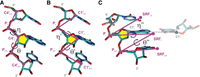
Structural representation of the pseudotorsional angles of RNA. (A) Definition of the η (eta: C4′i − 1, Pi, C4′i, Pi + 1) and the θ (theta: Pi, C4′i, Pi + 1, C4′i + 1) angles. (B) Definition of the η′ (eta′: C1′i − 1, Pi, C1′i, Pi + 1) and the θ′ (theta′: Pi, C1′i, Pi + 1, C1′i + 1) angles. (C) Definition of the η″ (eta″: SRFi − 1, Pi, SRFi, Pi + 1) and the θ″ (theta″: Pi, SRFi, Pi + 1, SRFi + 1) angles, where SRF stands for standard reference frame as implemented in DSSR (Lu et al. 2015).
Aiming to increase structural characterization, two other pseudotorsional angles have been defined, namely η′ − θ′, where the C4′ in η − θ was replaced by C1′ (Keating et al. 2011), and η″ − θ″, formed between the phosphate atoms and a standardized point in the nucleobase plane (Lu et al. 2015), according with the standard reference frame (SRF) as defined by Olson et al. (2001). η′ − θ′ was less explored even though in principle it seems more adequate than η − θ to fit the RNA backbone to X-ray electron density maps. The η″ − θ″ has the additional advantage that it contains information about the nucleobase orientation with respect to the RNA backbone, something not explicitly provided by the other two pairs of pseudotorsions. No comprehensive study has been published comparing the informational load of these pseudotorsional angles.
In recent years, the number of structures determined by X-ray crystallography (X-ray), nuclear magnetic resonance (NMR), or cryogenic electron microscopy (Cryo-EM) techniques, and available in public databases, has grown to the point where there is enough nonredundant data to extract statistical meaningful information. This allows us to compare isolated RNA molecules versus those bound to proteins, finding any potential bias related to the experimental sources of 3D structures, or to start adding sequence context to major conformers. Accordingly, in this work, we used an updated version of our veriNA3d R (Gallego et al. 2019) package to revisit the three pairs of pseudotorsional angles (η − θ, η′ − θ′, and η″ − θ″) as they emerge from nonredundant experimental structures available to date. We found that η − θ were the best pseudotorsions to describe RNA conformational space. We found 14 major states and detected nonnegligible differences in sampling of the different conformations, depending on the technique used to determine the structure. Finally, the presence of binding can lead to the exploration of typically empty regions of the conformational space, pointing toward the impact of induced fit in RNA–protein recognition and structural stabilization for the case of cations.
RESULTS AND DISCUSSION
The continuous growth in number of experimental RNA structures creates demands for periodic updates of the analyses based on structural data mining. Since the seminal work of Wadley et al. (2007), the number of deposited RNA structures in public databases like the PDB has increased by a factor of 4.5 (from 1333 in 2007 to 5978 in 2022) (Supplemental Fig. S2), providing a more complete picture of the RNA conformational space. We considered a complete data set containing all the structures and subdivisions in different subsets presented in Table 1. For example, structures were divided by the experimental techniques used to describe them. In the same way, the complete-data set was filtered in “naked” (naked-subset) and “interacting” (protein-subset, monovalent-subset, and divalent-subset) RNA fragments with the purpose of addressing the possible effects on RNA folding introduced by interacting partners ubiquitously found in biological contexts. Statistics on the number of nucleotides and RNA structures analyzed in this work are reported in Table 1. Finally, we analyzed the sequence dependence on the η − θ space and explored how to relate transitions in η − θ clusters with the rotation of canonical backbone torsions α, β, γ, δ, ε, ζ, and χ.
Summary of data sets used in this work and number of nucleotides and structures included in each of them
How much did the global η − θ RNA pseudotorsional space change from its conception to date?
The η − θ pseudotorsion (Fig. 1A), was classified according to the sugar-puckering conformation (North nonhelical and South) and analyzed following the same strategy reported by Pyle and coworkers on our complete-data set. Surprisingly, although we dramatically increased the number of analyzed structures (Table 1), our results for η − θ showed roughly the original distribution, except for two unreported HDRs for nonhelical nucleotides with North sugars (herein clusters numbered VII and VIII in Fig. 2A); and one new cluster in the η − θ/South space (cluster V, Fig. 2B). These results reveal only moderate changes in the sampled experimental η − θ space, indicating that either the RNA motifs space was already extensively explored by the X-ray structures available at that time, or that certain motifs remain elusive to experimental techniques.
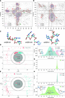
(A) η − θ from the complete-data set for nonhelical nucleotides with sugar conformation in North. Density contours of  (X = 1, 2, or 4; dark red, violet, and dark blue, respectively) highlight regions of the plots with a significant population
of nucleotides. Cluster or HDRs previously identified by Pyle and coworkers are labeled in red, while new clusters found in
this work appear in dark green. Black dashed lines delimit the region occupied by canonical helical A-form. (B) Same as (A) for nucleotides in South configuration. (C) Representative structure for each new cluster found. (D) Example of the stacking analysis for cluster I North. ρ and z components of the R-vector (Bottaro et al. 2014) between the given nucleobase and its 5′ (green) and 3′ (pink) neighboring nucleobases are shown. The inner space between
ellipses and dotted lines shows the region in which stacking occurs. (E) Same as (D) for cluster I South. (F) Interaction energy between the given nucleobase and its 5′ (green) and 3′ (pink) neighboring for cluster I North. (G) Direct interaction energy between the 5′ and 3′ nucleobases (one to three interactions) for cluster I North. (H) Same as (F) for cluster I South. (I) Same as (G) for cluster I South.
(X = 1, 2, or 4; dark red, violet, and dark blue, respectively) highlight regions of the plots with a significant population
of nucleotides. Cluster or HDRs previously identified by Pyle and coworkers are labeled in red, while new clusters found in
this work appear in dark green. Black dashed lines delimit the region occupied by canonical helical A-form. (B) Same as (A) for nucleotides in South configuration. (C) Representative structure for each new cluster found. (D) Example of the stacking analysis for cluster I North. ρ and z components of the R-vector (Bottaro et al. 2014) between the given nucleobase and its 5′ (green) and 3′ (pink) neighboring nucleobases are shown. The inner space between
ellipses and dotted lines shows the region in which stacking occurs. (E) Same as (D) for cluster I South. (F) Interaction energy between the given nucleobase and its 5′ (green) and 3′ (pink) neighboring for cluster I North. (G) Direct interaction energy between the 5′ and 3′ nucleobases (one to three interactions) for cluster I North. (H) Same as (F) for cluster I South. (I) Same as (G) for cluster I South.
The nonhelical North HDR described originally by Pyle and coworkers have either helical η (145° < η < 190°) or helical θ (190° < θ < 245°) values. Notably, the new clusters found in the η − θ North space (VII and VIII) have the same pattern. Therefore, all HDRs fall within the black dashed lines in Figure 2A, indicating that North nucleotides are usually located in the frontier of helical motifs. In contrast, the RNA nucleotides with sugar moieties in C2′-endo are, as expected, mostly found outside the helical region defined by black dashed lines in Figure 2B.
We investigated the structural composition of the identified clusters using the RMSD values for all trinucleotides of a given HDR, and a representative one was determined as the most similar to the others in the same region (the structure of all representative nucleotides is shown in Fig. 2C for new clusters reported herein and Supplemental Fig. S3). Using Pyle's similarity score (Wadley et al. 2007; see Table 2), we found that the new clusters VII–VIII in η − θ/North and cluster V in η − θ/South displayed high similarity percentages (98.8, 96.0, and 93.3, respectively), and therefore they are formed by a group of nucleotides with the same backbone conformation.
Summary of clusters’ similarities, and the number of PDBs in each cluster for η − θ conformational space
The stacking was described geometrically using the R-vector from base (i) to base (i ± 1) defined by the Bussi group (Bottaro et al. 2014) and energetically from thousands of QM calculations (see Materials and Methods). In this way, a systematic description of each HDR for both South and North sugar conformations was obtained (see Supplemental Table S1). The results in Figure 2D for clusters I in both North/South sugar conformations, display a range of energy that covers values from slightly repulsive stacking contributions to very stable ones (2 to −14 kcal/mol). Note how stacking interactions of the central nucleotide with its nearest neighbors are key for explaining conformations found in North cluster I (nHDR-I), while one to three interactions are the main players in stabilizing the structures found in cluster I/South (Fig. 2D). In this particular cluster, most trinucleotides come from internal-loops (49%) or junction-loops (20%), which are secondary motifs that contain several unpaired bases, some of them having flipped-out nucleobases as shown in Figure 2I.
The intramolecular hydrogen bond capability of the 2′OH group of the ribose in RNA (Darre et al. 2019), is another cornerstone contact among HDRs found far from the helical region. As described in detail in Supplemental Table S1, the 2′OH-phosphate interaction is a contact found prevalently in clusters I, II, and V in η − θ/North. This shows the versatile role of this interaction in stabilizing noncanonical motifs while also serving as a primary molecular switch contributing to specific protein–RNA recognition (Darre et al. 2019). Our detailed analysis of each HDR and the correlations of η − θ pseudotorsions with all backbone angles also allowed for a more general observation: all HDRs in the η − θ space are interconnected by a seemingly simple combination of torsional rotations (Fig. 3 for η and Supplemental Fig. S4 for θ). Transitions in the η axis appear mainly driven by changes in α, while transitions in θ depend on changes in ζ. This suggests an interpretation for RNA conformational transitions occurring at two levels: (i) a “coarse” level, which allows RNA to move between HDRs, and (ii) a “fine” level on how these movements translate to the all-atom space. This observation is developed below.
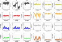
Distributions of real dihedral angles in the nucleotides i − 1 (panels on the left), i (mid-panels), and i + 1 (panels on the right), as a function of the pseudodihedral angle eta (η) in the central nucleotide i. Panels show: α (black), β (red), γ (blue), δ (green), ε (yellow), ζ (orange), ξ (gray), and the puckering phase (brown).
Global η′ − θ′ and η″ − θ″ RNA pseudotorsional space
The pseudotorsions η′ − θ′ and η″ − θ″ in their definition share similarities with the original η − θ torsions (Fig. 1B,C). In η′ − θ′ the C1′ atom is chosen instead of C4′, while in η″ − θ″ the SRF as defined by Olson and coworkers (Olson et al. 2001) is used to account for the relative orientation of the base with respect to the backbone. It should be noted that the location of the SRF depends upon the width of base-pair C1′ − C1′ spacing and the pivoting of complementary bases in the base-pair plane, and hence to analyze single-stranded RNA an idealized base-pair reference is needed.
A first inspection of the η′ − θ′ space (Supplemental Fig. S5A,B) revealed a very similar distribution to the one provided by η − θ, but with lower power to discriminate backbone substates as less clusters are visible in the North/South planes (nine in η′ − θ′ vs 13 in η − θ, compare Fig. 2 with Supplemental Fig. S5). Despite its reduced descriptive power at the backbone level, the η′ − θ′ pseudotorsional space might be advantageous for mapping X-ray models to their electron density maps, given that C1′ is used as a key reference atom to fit the experimental densities into molecular models (Keating and Pyle 2010; Gruene and Sheldrick 2011; Keating et al. 2011; Li et al. 2019). Coarse-grained models for RNA (Dans et al. 2019) based on η′ − θ′ could also benefit over η − θ since the C1′ atom is used to define the major/minor groove in curvilinear helicoidal coordinates (Lavery et al. 2014); therefore, the grooves’ dimensions would have a direct readout.
To our knowledge, no data mining of PDB has been done to date using the η″ − θ″ pseudotorsional space. In our data sets, the η″ − θ″ space looks similar to η − θ and η′ − θ′ (Supplemental Fig. S5C,D), but less defined clusters are observed (eight in total). As a result, the power to discriminate backbone substates is even
lower than the η′ − θ′ one, as North clusters I to IV belong to the same HDR with contour  . Each cluster is then a more heterogenic mixture of backbone conformations, and hence η″ − θ″ appears to be not so useful to describe and understand substate diversity as found experimentally.
Additionally, we analyzed the power of each pseudotorsion in explaining the secondary motifs displayed by RNA molecules. This was quantified by analyzing the composition of secondary motifs (stem, stem-end, internal-loop, hairpin-loop, junction-loop, ss-non-loop, and bulge) that are present in the defined clusters. According to Supplemental Figure S6, there are no clear advantages of one pseudotorsion over the others in separating the secondary motif among clusters. Hairpin loops are present in all the clusters but are more abundant in cluster II/North for the three angles. In the same way, internal-loops are more present in South, cluster III in η − θ and cluster XI in η′ − θ′/η″ − θ″. In summary, even if the η′ − θ′ definition might have some advantages in terms of modeling, the traditional η − θ space is preferable to describe the conformational space accessible by the RNA backbone.
Experimental techniques describing RNA conformations
Originally, only high-resolution structures obtained by X-ray crystallography were used to analyze the η − θ space (Wadley et al. 2007). However, to date, an important number of RNA structures were determined by means of solution NMR, and more recently by Cryo-EM which has reached a resolution close to that of an X-ray while allowing for the determination of huge RNA complexes (Natchiar et al. 2017). We then divided the complete-data set into three subsets, one for each method, in order to analyze their contributions and limits: xray-subset, nmr-subset, and em-subset (see Materials and Methods). As shown in Table 1, a significant number of nucleotides can still be analyzed despite the division performed.
The xray-subset (Fig. 4A,B), although being dramatically enlarged in the number of structures, reproduces well Pyle's η − θ space (Wadley et al. 2007). The em-subset (Fig. 4C,D) and nmr-subset (Fig. 4E,F) show new clusters VII/VIII in the North plane and cluster V in the South plane. Clusters VII–VIII in η − θ/North are mostly exclusively populated by trinucleotides found in large ribosomal complexes that could have been determined with atomic resolution only recently (Nakane et al. 2020). Apart from these two new clusters, trinucleotides in the em-subset, extracted from only 32 PDB structures (Table 1), reproduce by themselves all the conformational substates observed in the complete-data set. Remarkably, ribosomes seem to exploit geometrically and energetically all the possible backbone substates to achieve their complex 3D folded structures that in turn depend on RNA–protein interactions. Interesting results are obtained when analyzing the pseudotorsional space revealed by solution NMR experiments (nmr-subset). As shown in Figure 4E,F, only certain conformations seem to be detected when using this technique (clusters II–III–IV–VI in North and IV–V in South), where large deviations from the canonical η − θ values are not frequently sampled. The new cluster V/South described herein for the complete-data set (Fig. 2B) is mainly composed by structures determined using NMR. Furthermore, focusing on the nmr-subset, the large and heterogeneous cluster IV/South can be divided into two clearly distinct populations (Fig. 4F).
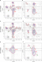
η − θ conformational space as detected by each experimental technique. Results are divided into North (panels on the left) or South (panels on the right) sugar conformations. Density contours of  (X = 1, 2, or 4; dark red, violet, and dark blue, respectively) highlight regions of the plots with a significant population
of nucleotides. Black dashed lines delimit the region occupied by canonical helical A-form (those structures are removed from
the analyses as described in the Materials and Methods section). Cluster numbers are identified in red or dark green when
they were not seen in the complete-data set depicted in Figure 2. (A) Densities and cluster analysis of the xray-subset for central nucleotides with sugars in North. (B) Same as (A) for South conformations. (C,D) are the same as (A) and (B) for the em-subset. (E,F) are the same as (A) and (B) for the nmr-subset.
(X = 1, 2, or 4; dark red, violet, and dark blue, respectively) highlight regions of the plots with a significant population
of nucleotides. Black dashed lines delimit the region occupied by canonical helical A-form (those structures are removed from
the analyses as described in the Materials and Methods section). Cluster numbers are identified in red or dark green when
they were not seen in the complete-data set depicted in Figure 2. (A) Densities and cluster analysis of the xray-subset for central nucleotides with sugars in North. (B) Same as (A) for South conformations. (C,D) are the same as (A) and (B) for the em-subset. (E,F) are the same as (A) and (B) for the nmr-subset.
Being based on completely different approaches and physical observables, which make comparisons rather difficult, the main differences among these three methods might arise from features like the experimental temperature at which data collection is produced. While Cryo-EM typically cools down the sample between 4 K (liquid helium cryogen) and 77 K (nitrogen, propane, or ethane coolers) (Doerr 2017), the structures from the xray-subset were collected at 112 ± 44 K and NMR ones at near NTP conditions 293 ± 28 K. Above a given temperature threshold, thermal fluctuations of RNA molecules in solution might be preventing the transient stabilization of some extreme and less stable backbone substates. Consequently, some substates detected by Cryo-EM and X-ray may not be captured when performing NMR experiments. Additionally, the use of smaller X-ray structures to fit large and/or multimeric Cryo-EM densities could be another important reason behind the similarity found between both data sets in terms of eta–theta. Other differences between these three methods might arise from the different size of the RNA molecules in each of the data sets. Apparently, this should not be relevant as the average chain length of the analyzed structures is very similar between NMR and X-ray data sets (26 and 34 residues on average, respectively, while it is 323 for the em-subset). However, a closer look into our data sets indicates that both the X-ray and Cryo-EM subsets contain several long RNA chains such as ribosomes with thousands of nucleotides that can sample all the conformational space of the RNA backbone, whereas the longest structure in the NMR set is 155 residues (PDB ID: 2N1Q) and contains mostly A-form RNA. Apparently, the longer an RNA molecule is, the easier it is to explore alternative nonhelical conformations, but this phenomenon could also be influenced by the contacts with proteins, which is explored hereafter.
How do proteins affect the RNA η − θ space?
We divided the complete-data set into “naked” RNA and protein-bound RNA. This allowed for the analysis of the intrinsic or “naked” conformations that RNA could adopt (naked-subset) and the effect produced by proteins (protein-subset). The η − θ plots for North puckering (Fig. 5) reveal that, while the protein-subset (RNA with a protein residue closer than 5 Å) roughly resembles the complete-data set, the naked-subset shows a nucleotide distribution confined to the helical region neighborhood (clusters III, IV, and VI). Clusters I/III/IV show a noticeable reduction in their population and no HDR are found near θ values of ∼0° (new cluster VIII in the complete-data set). These differences are an evident consequence of the divergent η − θ density distributions in the absence and presence of proteins. That is, the density of the naked-subset biases the sampling of the complete-data set toward near-helical regions, while proteins preferentially enrich conformations far from the helical center. Summarizing, these results indicate that proteins can stabilize North pucker RNA segments with η and θ values far from the helical conformation, which are less sampled in “naked” RNA. In the case of South puckering nucleotides, the absence of proteins enriches cluster IV in the helical region, splitting the cluster into two sub-HDR regions.
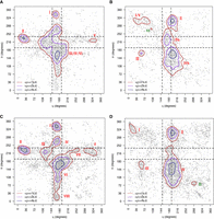
η − θ conformational space described by the naked-subset and protein-subset. Results are divided into nonhelical North (panels
on the left) or South (panels on the right) sugar conformations. Density contours of  (X = 1, 2, or 4; dark red, violet, and dark blue, respectively) highlight regions of the plots with a significant population
of nucleotides. Black dashed lines delimit the region occupied by canonical helical A-form (those structures are removed from
the analyses as described in the Materials and Methods section). Cluster numbers are identified in red or dark green when
they were not seen in the complete-data set depicted in Figure 2. (A) Densities and cluster analysis of the naked-subset for central nucleotides with sugars in North. (B) Same as (A) for South conformations. (C,D) are the same as (A) and (B) for the protein-subset.
(X = 1, 2, or 4; dark red, violet, and dark blue, respectively) highlight regions of the plots with a significant population
of nucleotides. Black dashed lines delimit the region occupied by canonical helical A-form (those structures are removed from
the analyses as described in the Materials and Methods section). Cluster numbers are identified in red or dark green when
they were not seen in the complete-data set depicted in Figure 2. (A) Densities and cluster analysis of the naked-subset for central nucleotides with sugars in North. (B) Same as (A) for South conformations. (C,D) are the same as (A) and (B) for the protein-subset.
How do cations affect the RNA η − θ space?
To analyze the effect of the direct contact of monovalent (Na+ and K+) and divalent (Ca2+, Mg2+, and Mn2+) cations on η − θ, we filtered the complete-data set, keeping only those trinucleotides with at least one cation closer than 5 Å. Cation binding to RNA can serve to stabilize a specific 3D structure, perform a catalytic role (Hendrix et al. 2005) and is a requirement for folding (Nguyen et al. 2019). As previously observed (see Table 1), structures containing divalent cations (particular Mg2+) are significantly more abundant than the ones containing Na+ and K+ (Stefan et al. 2006) (although the assignment is not always accurate [Auffinger et al. 2011]), while it was proposed that the formation of RNA-structural motifs seems to be Mg2+ independent, since this cation binds preferentially to RNA regions others than the well-established secondary conformations (hairpins, internal-loops, junctions, etc.) (Hsiao et al. 2009). Figure 6 and Supplemental Table S2 highlight the main results observed for the monovalent- and divalent-subsets upon removal of those helical nucleotides. All clusters of the complete-data set (Fig. 2A,B) are still present when only the structures with cations are retained (Fig. 6A), several of them being denser (clusters I, III, V, VII, and VII in both North nonhelical and South), and even new minor clusters appeared that were not significant at the complete-data set level (Fig. 6B,C). Enhanced clusters involve backbone conformations far from the helical regions, and new ones are located at extreme η values (<72° and >300°). This supports the structural role for a significant portion of the cations determined experimentally that are particularly enriched around backbone conformations highly distorted, stabilizing peculiar RNA motifs. We quantified this observation by computing the number of trinucleotides in helical and nonhelical regions with and without monovalent and divalent cations (Supplemental Table S2). Although RNA is mostly found not to be surrounded by cations (from 89.7% to 97.3% of the time), a slight enrichment of divalent and monovalent cations is seen going from helical to nonhelical regions (2.4% for divalent cations and 1.0% for monovalent).
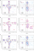
η − θ conformational space described by the monovalent-subset and divalent-subset. Results are divided into nonhelical North (panels
on the left) or South (panels on the right) sugar conformations. Density contours of  (X = 1, 2, or 4; dark red, violet, and dark blue, respectively) highlight regions of the plots with a significant population
of nucleotides. Black dashed lines delimit the region occupied by canonical helical A-form (those structures are removed from
the analyses as described in the Materials and Methods section). (A) Densities and cluster analysis of the both types of cations together (monovalent in pink dots and divalent in turquoise)
over the clusters obtained for the complete-data set. (B) Clusters obtained by using only the monovalent-subset. (C) Idem than (B) using the divalent-subset.
(X = 1, 2, or 4; dark red, violet, and dark blue, respectively) highlight regions of the plots with a significant population
of nucleotides. Black dashed lines delimit the region occupied by canonical helical A-form (those structures are removed from
the analyses as described in the Materials and Methods section). (A) Densities and cluster analysis of the both types of cations together (monovalent in pink dots and divalent in turquoise)
over the clusters obtained for the complete-data set. (B) Clusters obtained by using only the monovalent-subset. (C) Idem than (B) using the divalent-subset.
Sampling of the η − θ space is nucleobase dependent
The large number of nucleotides in each cluster allows for a reasonable analysis on the sequence dependencies in the η − θ space. Notable differences are observed when the complete-data set η − θ map for North sugar rings is decomposed into nucleobase identity as evidenced in Figure 7. Despite fluctuations in their relative populations, clusters nearby the helical region (III, IV, and VI), and cluster II are clearly observed for all four nucleobases, as well as South clusters II and III. However, cluster I/North is depopulated of adenine (<12%), cluster V is almost exclusive of guanine (present at that position more than 50% of the time), and uracil is almost absent in clusters V and VII (with an occurrence below 9% and 7%, respectively). Considering that these later clusters are more populated in protein–RNA complexes (see previous sections), this result suggests that the nucleobase-dependent sampling of the η − θ space is, in part, a consequence of sequence-specific protein–RNA contacts. Furthermore, the presence of purines in the trinucleotide motif displayed as logo-plots is slightly dominant outside the helical region in North, GAA, AAG, GGA, and GAA being the most common sequences for clusters II, IV, IV, and VIII. In the case of South sugar rings, nucleobase dependence has been also observed to some extent, with cluster V mainly populated by uracil and adenine (52% and 27%, respectively), and adenine being mainly responsible for cluster IV (52% of the time).
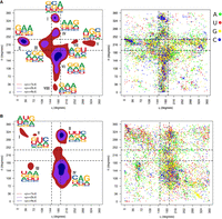
η − θ conformational space of the complete-data set. Results are divided into nonhelical North (top-panels) or South (bottom-panels) sugar conformations. Density contours of  (X = 1, 2, or 4; dark red, violet, and dark blue, respectively) highlight regions of the plots with a significant population
of nucleotides. Black dashed lines delimit the region occupied by canonical helical A-form (those structures are removed from
the analyses as described in the Materials and Methods section). Cluster numbers are identified in black in the left panels. (A) The panel on the left shows densities and sequence logo-plots of the complete-data set for sugars in North. The panel on the right shows the corresponding dot-plot with adenine (green), uracil (red), guanine (yellow), and cytosine (blue). (B) Same as (A) for South conformations.
(X = 1, 2, or 4; dark red, violet, and dark blue, respectively) highlight regions of the plots with a significant population
of nucleotides. Black dashed lines delimit the region occupied by canonical helical A-form (those structures are removed from
the analyses as described in the Materials and Methods section). Cluster numbers are identified in black in the left panels. (A) The panel on the left shows densities and sequence logo-plots of the complete-data set for sugars in North. The panel on the right shows the corresponding dot-plot with adenine (green), uracil (red), guanine (yellow), and cytosine (blue). (B) Same as (A) for South conformations.
A small set of torsional perturbations applied to a helical structure fully explain the RNA conformational diversity
All the North η − θ clusters fall into the space of helical η (∼160°) or helical θ (∼215°) (see the red lines in all our η − θ maps). Therefore, in most cases the backbone can move from one cluster to another just by rotating η or θ. For example, to go from the HDR-II (η = 30°, θ = 215°) to the HDR-III (η = 110°, θ = 215°), the backbone only needs to move along the η axis. To acquire insight on the specific torsion changes coupled to η and θ, average values of α, β, γ, δ, ε, ζ, χ, and puckering were calculated for η and θ values in 5° windows. This was done for the central, and for the first 5′- and 3′-neighbors. Figure 3 for η and Supplemental Figure S4 for θ suggests that simple combinations of specific torsional per-turbations encode the transitions between nHDRs. We have shown before that the torsions of η and θ can be traced by the movements of the real dihedral angles α, β, γ, δ, ε, ζ, χ, and puckering. Considering the η direction (Fig. 3), discrete perturbations in ε, ζ, and puckering in the 5′-neighbor, and in α and γ in the central nucleotide result in the sequential transitions: nHDR-II ↔ nHDR-III ↔ helical ↔ nHDR-VII ↔ nHDR-V. Considering the θ direction (Supplemental Fig. S4), perturbations in α, γ, and ζ for the central nucleotide, and in α, γ, and puckering for the 3′-neighbor, explain the sequential transitions: nHDR-I ↔ nHDR-IV ↔ helical ↔ nHDR-VI ↔ nHDR-VIII. These results suggest that moving from the helical conformation to any of the nHDRs can be achieved by specific combinations of discrete torsional perturbations. This result implies that the complete North puckering RNA conformational space can be rationalized as a helical structure plus a small set of specific combinations of torsional perturbations.
Conclusions
We explored here the conformational space of the “experimental” RNA backbone using our package veriNA3d (Gallego et al. 2019). The large size of the database allowed dividing the data into different subsets, exploring relationships that were not addressed before, such as the effect of proteins on the RNA backbone, or intrinsic differences due to the source of experimental structures. In addition, alternatives to η − θ to study the backbone conformation have been used, such as the η′ − θ′ (which uses the C1′ instead of C4′) and the η″ − θ″ (which uses a standardized point in the base plane instead of the C4′). We explored these alternative maps but found out that they tend to form less clusters and are more heterogeneous, so we focused our analysis on the original η − θ space.
Quite surprisingly, the updated η − θ maps show overall a similar general distribution to that found in Pyle's 2007 study (Wadley et al. 2007). However, we detected the presence of three small new clusters not reported previously. In general, the X-ray and Cryo-EM subsets show almost equivalent η − θ maps, while the NMR-subset is much more limited, covering only the clusters close to the helical A-form. One plausible explanation is that X-ray and Cryo-EM data sets include very large structures with thousands of nucleotides (e.g., ribosomes) and proteins that expand the conformational space that can be sampled by RNA in nonhelical regions. Overall, it is clear that complementary sources of data are needed to fully recover the landscape of RNA backbone conformations.
Comparing samplings in naked-subset and protein-subset, we find evidence that protein contacts allow the RNA backbone to adopt the most extreme conformations. This agrees with previous findings in which proteins are shown to modulate the RNA conformation through contacts with the 2′OH (Darre et al. 2019). By their side, a significant portion of monovalent and divalent cations also appears, stabilizing backbone conformations far from the helical regions.
We also find that the transitions between clusters can be traced by the rotation of specific dihedral angles, and only a few changes are necessary to go from one cluster to another. Given that the η − θ maps are particularly interesting for coarse-grained applications in modeling RNA (Dans et al. 2019), our finding introduces a new way of moving in the η − θ space by using the real dihedral angles.
MATERIALS AND METHODS
Atomic-resolution structural data and RNA equivalence classes
The primary source of RNA-structural data is the PDB. This database is highly redundant and is also biased toward those structures that are determined more easily experimentally, which means that before starting with any desired analysis, some degree of filtering of structures deposited in the PDB is required to obtain a nonredundant set (Leontis and Zirbel 2012). The Leontis group classified types of redundancy and they generate weekly lists of “Equivalence Classes” of RNA on their website (http://rna.bgsu.edu/rna3dhub/nrlist). Each Equivalence Class contains all the RNA redundant chains and a representative structure. Equivalence Classes contain RNA chains rather than complete PDB IDs. A nonredundant set of structures is provided by the list of Equivalence Class Representatives. They offer different lists of X-ray structures according to a resolution threshold, and an additional list called “All” including all experimental conditions. For our purpose, the “All” list was used here, as defined in the release version 3.134.
Nonredundant data sets
From the Leontis list, different sets of nonredundant structures were obtained: complete-data set using all Equivalence Classes, protein-subset when the RNA is in contact with a protein, monovalent/divalent-subsets when in contact with cations (K+/Na+ and Ca2+/Mg2+/Mn2+, respectively) and naked-subset which contains free RNA. In addition, the complete-data set was also divided into three additional subsets representing the determination techniques: xray-subset, nmr-subset, and em-subset for X-ray, NMR, and Cryo-EM techniques, respectively. For the X-ray and Cryo-EM structures, a resolution threshold of 2.4 Å was used to ensure a correct description of the sugar puckering (Jain et al. 2015). We considered only RNA chains with three or more nucleotides, the minimum number to measure the eta–theta parameters. Next, all the nucleotides were analyzed and divided into two sets according to their puckering state (North or South). North nucleotides (C3′-endo) were selected according to these criteria: δ = 84° ± 30°; phase between −18° and 54°; and Dp distance (base-phosphate perpendicular distance, defined in Jain et al. 2015) >2.9 Å. South nucleotides (C2′-endo) were defined with: δ = 147° ± 30°; phase between 126° and 198°; and Dp distance ≤2.9 Å. Nucleotides that lacked atoms or whose bond distances exceed the threshold of 2 Å were considered as “broken” and excluded. Nucleotides obtained using X-ray with the phosphate or the C4′/C1′ atom with B-factor over 60 were also excluded (Keating et al. 2011). The final nucleotides in the data set were restricted to the A, U, G, and C residues that have a complete backbone starting from the sugar of the “i − 1” nucleotide (5′ neighbor) to the sugar of the “i + 1” (3′ neighbor).
Definitions and calculations
Once the list of structures was compiled, we computed the geometrical analysis of the RNA backbone. η − θ and other dihedrals were defined as in Wadley et al. (2007). Puckering was measured as in Westhof and Sundaralingam (1985). Stacking was represented geometrically using the R vectors defined by Bottaro et al. (2014) and quantified using a QM approach (see below). In Bottaro's approach, the z-axis measures the vertical distance between two nucleobases having their glycosidic bond (angle ξ) in the canonical anticonformation (Bottaro et al. 2014). According to this reference frame, the central nucleobase of a canonical trinucleotide will have positive values of z toward the 5′ side and negative values toward the 3′ side. The calculation of the distance between points in the η − θ map and the scoring of η − θ clusters were carried out as described in Wadley et al. (2007). RMSD, εRMSD (Bottaro et al. 2014), torsions, and distances were computed in R using our package veriNA3d (Gallego et al. 2019). RMSD calculations included backbone atoms from C4′i − 1 to C4′i + 1 or C1′i − 1 to C1′i + 1 in the case of η′ − θ′. For the other nucleotide descriptors, such as base pairing and η″ − θ″, DSSR software was used (Lu et al. 2015). See Figure 1 for a structural representation of the pseudotorsional angles used to characterize RNA at the trinucleotide level.
Ramachandran-like plots
The η − θ plot of North nucleotides revealed a large, highly populated region near its center (Supplemental Fig. S1). This region contains nucleotides with a backbone conformation typical of an A-RNA helix, so we refer to it as the helical region. It has a density that is almost two orders of magnitude higher than any other region of the η − θ map. To study the surrounding regions with precision, we separated the set of North nucleotides into helical and nonhelical nucleotides like in Wadley's work (Wadley et al. 2007). Separate η − θ maps were so constructed for the nonhelical North nucleotides and all South nucleotides. The same approach was applied to η′ − θ′ and η″ − θ″ plots. For each plot, the density was measured using a kernel density estimation (KDE), with 361 × 361 grid points and a bandwidth = 40. These parameters were chosen in order to exactly match the original results obtained by Pyle and coworkers using their data set published in 2007 (Wadley et al. 2007). From the densities at each point of the η − θ map, the mean (<ρ>) and standard deviation (σ or s.d.) were calculated and contour levels at <ρ> + X • σ (using X = 1, 2, and 4) were added to define high-density regions (HDRs) or clusters. We defined as a cluster or HDR, trinucleotides grouped locally whose estimated density values were above <ρ> + 2 s.d. (i.e., clusters I, II, III, IV, and VI in Fig. 2A). We also defined as an HDR or cluster, a given isolated group of trinucleotides having a density above <ρ> + 1 s.d. (clusters V, VII, and VIII in Fig. 2A).
Stacking energy calculation
At the trinucleotide level, three combinations of stacking interactions were computed: the central base (i) with the nucleotide at its 5′-side (i − 1), the central base with the nucleotide at its 3′-side (i + 1), and (i − 1)-to-(i + 1) direct interaction that does not involve the central base. To compute the stacking energy, the backbone of each trinucleotide was removed and replaced by a methyl group. Then the geometry of the individual bases was replaced by that optimized at the MP2/cc-pVTZ level of theory (Woon and Dunning 1993). The optimization was done on isolated nucleobases, defining an “ideal” geometry for each of the canonical nucleobases (A, C, G, and U). At the trinucleotide level, the coordinates of each of the three nucleobases were then replaced by their “ideal” version, based on the overlap of the ring atoms N1, C2, N3, C4, C5, C6 for pyrimidines, and N1, C2, N3, C4, C5, C6, N7, C8, N9 for purines. Quantum mechanical energies were calculated at the dispersion-corrected (Grimme et al. 2010, 2016) DFT level B3LYP-D3(BJ) with the double-polarized def2-TZVPP basis set (Weigend and Ahlrichs 2005), and interaction energies were corrected by the basis-set superposition error (BSSE) following the Boys and Bernadi counterpoise method (Gutowski et al. 1993).
SUPPLEMENTAL MATERIAL
Supplemental material is available for this article.
Footnotes
-
↵5 Co-first authors.
-
Article is online at http://www.rnajournal.org/cgi/doi/10.1261/rna.079821.123.
- Received September 1, 2023.
- Accepted September 1, 2023.
This article is distributed exclusively by the RNA Society for the first 12 months after the full-issue publication date (see http://rnajournal.cshlp.org/site/misc/terms.xhtml). After 12 months, it is available under a Creative Commons License (Attribution-NonCommercial 4.0 International), as described at http://creativecommons.org/licenses/by-nc/4.0/.