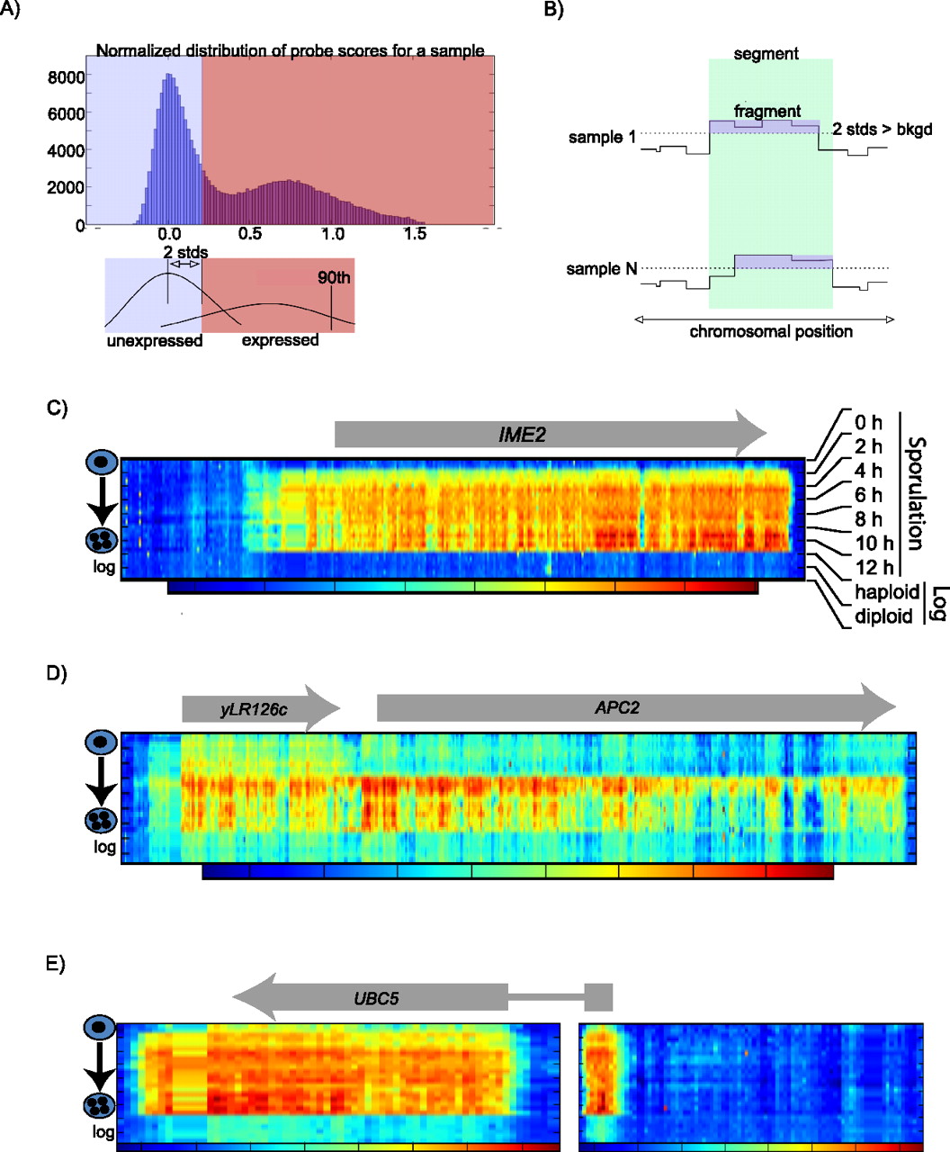
Segmentation pipeline. (A) For each array, the background was calculated from the histogram of normalized probe scores on all probes on that array (top). The signal was assumed to come from either expressed or unexpressed distributions. The background cut-off was taken as two standard deviations from the median of the unexpressed distribution (bottom). This first step of the pipeline establishes “fragments” of expression for each array. (B) To determine a constant segment of expression across samples, the union of the fragments was created as the second step of the pipeline. This established the segment boundaries and allowed an analysis of architecture changes across meiosis. (C) Heat map of a segment corresponding to a conventional gene (IME2) that is expressed specifically during meiosis. The x axis represents the genomic coordinates with the start and end of the arrow indicating the approximate location of the annotated start and stop codons, respectively. The array signals (three biological replicates for each time point) are stacked along the y axis with the beginning of meiosis at the top. The final six layers are from log-phase haploid and diploid cells. The heat map is generated for each segment individually, with the coloring indicated in the bar directly below the heat map (red and blue denote high and low signal, respectively). (D) Heat map of a single computationally defined segment containing yLR126c and APC2 as an example of a segment that contains more than one annotated ORF. (E) Heat map of a single annotated ORF (UBC5) that was split between two segments.